Getting Started

The main API consists of WENOScheme, MultiphaseWENOScheme, and WENO_step!. The user must define the grid and the initial conditions themselves.

WENOScheme() is used to create a WENO scheme structure containing all the necessary information for the WENO method, while WENO_step!() performs one step of the time integration using the WENO-Z method and a 3rd-order Runge-Kutta method. Refer to the docstrings to see the available options for each function.

WENOScheme takes two independent keywords: form selects which equation is solved (:conservative for $\partial_t u + \nabla\cdot(\mathbf{v}u) = 0$, :nonconservative for $\partial_t u + \mathbf{v}\cdot\nabla u = 0$), and stag selects where the velocity lives (false for collocated with u, true for face-staggered). All four combinations are fifth-order accurate; see Background for why this package treats them as separate choices rather than one implying the other.

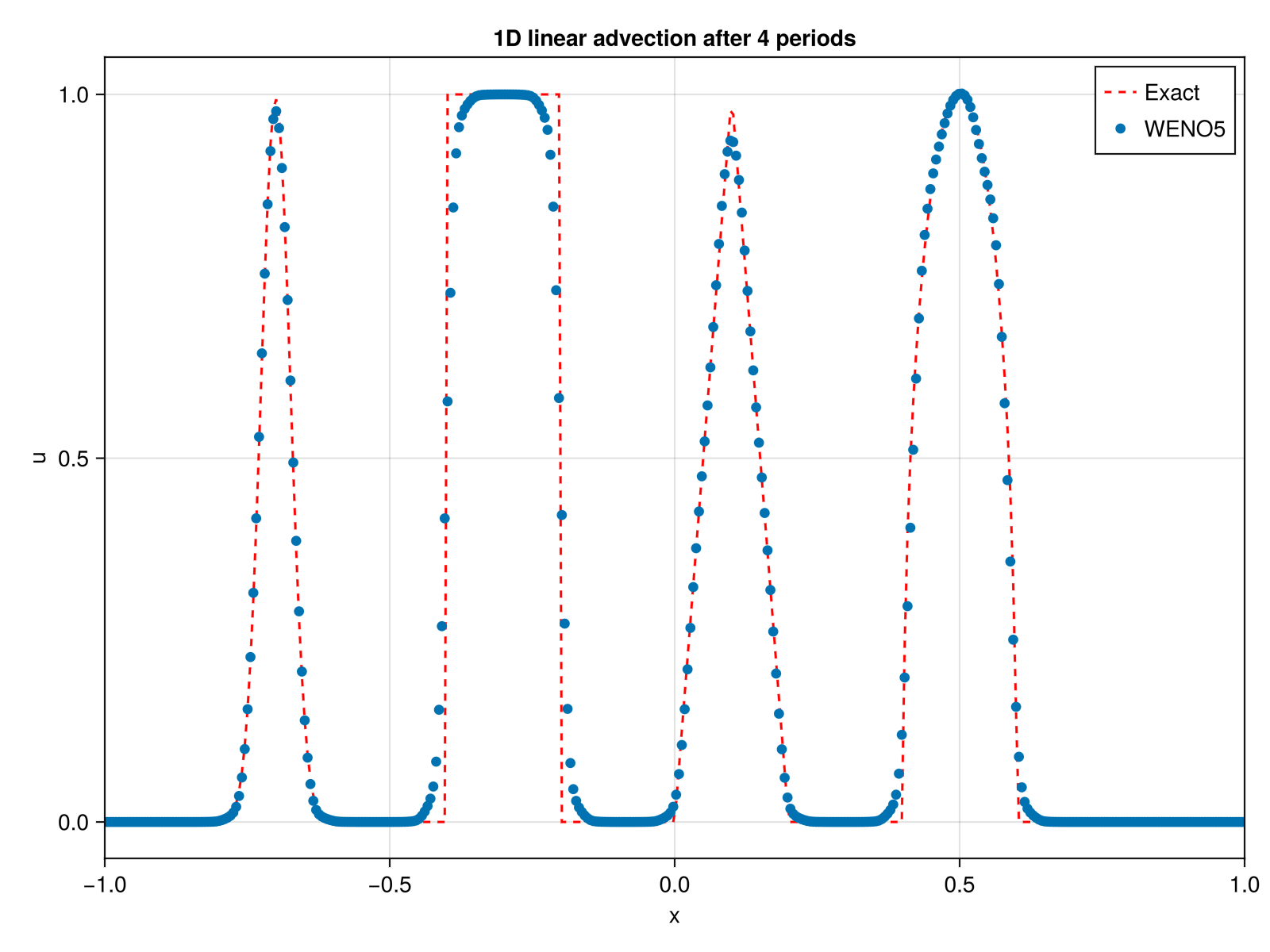
Here is a simple example of how to use FiniteDiffWENO5.jl to solve the 1D advection equation using the conservative form on a staggered grid. For more examples, please refer to the folder examples in the repository or the tests in the test folder.

using FiniteDiffWENO5

nx = 400

x_min = -1.0
x_max = 1.0
Lx = x_max - x_min

x = range(x_min, stop = x_max, length = nx)

# Courant number
CFL = 0.4
period = 4

# Parameters for Shu test
z = -0.7
δ = 0.005
β = log(2) / (36 * δ^2)
a = 0.5
α = 10

# Functions
G(x, β, z) = exp.(-β .* (x .- z) .^ 2)
F(x, α, a) = sqrt.(max.(1 .- α^2 .* (x .- a) .^ 2, 0.0))

# Grid x assumed defined
u0_vec = zeros(length(x))

# Gaussian-like smooth bump at x in [-0.8, -0.6]
idx = (x .>= -0.8) .& (x .<= -0.6)
u0_vec[idx] .= (1 / 6) .* (G(x[idx], β, z - δ) .+ 4 .* G(x[idx], β, z) .+ G(x[idx], β, z + δ))

# Heaviside step at x in [-0.4, -0.2]
idx = (x .>= -0.4) .& (x .<= -0.2)
u0_vec[idx] .= 1.0

# Piecewise linear ramp at x in [0, 0.2]
# Triangular spike at x=0.1, base width 0.2
idx = abs.(x .- 0.1) .<= 0.1
u0_vec[idx] .= 1 .- 10 .* abs.(x[idx] .- 0.1)

# Elliptic/smooth bell at x in [0.4, 0.6]
idx = (x .>= 0.4) .& (x .<= 0.6)
u0_vec[idx] .= (1 / 6) .* (F(x[idx], α, a - δ) .+ 4 .* F(x[idx], α, a) .+ F(x[idx], α, a + δ))


u = copy(u0_vec)

# Periodic boundaries on both faces.
# staggering = true means that the advection velocity is defined on the sides of the cells and should be of size nx+1 compared to the scalar field u.
# Multithreading to false means that the computations will be done on a single thread.
# Set to true to enable multithreading if the Julia session was started with multiple threads (e.g. `julia -t 4`).
weno = WENOScheme(u; form = :conservative, boundary = (PeriodicBC(), PeriodicBC()), stag = true, multithreading = false)

# advection velocity with size nx+1 for staggered grid (here constant)
a = (; x = ones(nx + 1))

# grid size
Δx = x[2] - x[1]
Δt = CFL * Δx^(5 / 3)

tmax = period * (Lx + Δx) / maximum(abs.(a.x))

t = 0

while t < tmax
    # take as input the scalar field u, the advection velocity a as a NamedTuple,
    # the WENO scheme struct weno, the time step Δt and the grid size Δx
    WENO_step!(u, a, weno, Δt, Δx)

    t += Δt

    if t + Δt > tmax
        Δt = tmax - t
    end
end

f = Figure(size = (800, 600), dpi = 400)
ax = Axis(f[1, 1], title = "1D linear advection after $period periods", xlabel = "x", ylabel = "u")
lines!(ax, x, u0_vec, label = "Exact", linestyle = :dash, color = :red)
scatter!(ax, x, u, label = "WENO5")
xlims!(ax, x_min, x_max)
axislegend(ax)
display(f)

which outputs:

Boundary conditions

Use PeriodicBC() for wrapped domains, ExtrapolateBC() for open boundaries, and PrescribedInflowBC(value) to prescribe the exterior state only where the normal velocity enters the domain. In 2D, boundary tuples are ordered as (west, east, bottom, top). value may be a scalar or a vector along the face.

bc = AdvectionBC(
    west = PrescribedInflowBC(fill(300.0, ny)),
    east = ExtrapolateBC(),
    bot = ExtrapolateBC(),
    top = ExtrapolateBC(),
)
weno = WENOScheme(u; form = :conservative, boundary = bc, stag = true)

Advecting multiple fields

If you have multiple scalar fields (e.g. different chemical components) that share the same velocity, you can advect them all in a single call by passing a tuple of arrays. The same WENOScheme buffers are reused for each field, so there is no extra memory overhead.

Each field gets its own u_min / u_max bounds for the Zhang-Shu limiter, passed as tuples matching the number of fields.

using FiniteDiffWENO5

nx = 200
ny = 200
Lx = 1.0
Δx = Lx / nx
Δy = Lx / ny

# Three chemical components with different initial distributions
c1 = rand(nx, ny)    # component 1
c2 = zeros(nx, ny)   # component 2
c3 = ones(nx, ny)    # component 3

# Shared velocity field
v = (; x = ones(nx, ny), y = 0.5 .* ones(nx, ny))

# Create the WENO scheme from any one of the fields (they must all have the same size/type).
# Independent tracers do not sum to anything meaningful, so either form is valid here;
# non-conservative is used since the velocity is already collocated.
weno = WENOScheme(c1; form = :nonconservative, boundary = (2, 2, 2, 2), stag = false)

Δt = 0.7 * min(Δx, Δy)^(5 / 3)

# Advect all three fields in one call
WENO_step!((c1, c2, c3), v, weno, Δt, Δx, Δy;
    u_min = (0.0, 0.0, 0.0),
    u_max = (1.0, 1.0, 1.0))

This also works with KernelAbstractions and Chmy backends — just pass the extra backend/grid arguments as usual:

# KernelAbstractions
WENO_step!((c1, c2, c3), v, weno, Δt, Δx, Δy, backend;
    u_min = (0.0, 0.0, 0.0), u_max = (1.0, 1.0, 1.0))

# Chmy
WENO_step!((c1, c2, c3), v, weno, Δt, Δx, Δy, grid, arch;
    u_min = (0.0, 0.0, 0.0), u_max = (1.0, 1.0, 1.0))

Material fractions

The tuple call with a WENOScheme reconstructs each field independently. It is useful for unrelated tracers, but it does not preserve a pointwise sum. Use MultiphaseWENOScheme when the fields are fractions of one material composition:

phases = (ϕ1, ϕ2, 1 .- ϕ1 .- ϕ2)
boundary = ntuple(_ -> PeriodicBC(), 4)
scheme = MultiphaseWENOScheme(phases; boundary = boundary, stag = true)
WENO_step!(phases, velocity, scheme, Δt, Δx, Δy)

Every input cell must initially satisfy 0 ≤ ϕₖ ≤ 1 and Σₖϕₖ = 1. The operator does not repair invalid input or renormalise after a step. Bound preservation requires a stable explicit CFL, as for the scalar SSP-RK3 operator. Interfaces remain diffuse and are transported as continuous fractions.

A prescribed inflow supplies the complete composition:

west = PrescribedInflowBC((0.2, 0.3, 0.5))
boundary = AdvectionBC(
    west = west, east = ExtrapolateBC(),
    bot = PeriodicBC(), top = PeriodicBC())