3D Subduction example

This is a 3D subduction example for LaMEM.jl that illustrates how to use the julia interface. This is very similar to the setup described by Schellart and coworkers in a 2007 nature paper in which they demonstrate that toroidal flow changes the slab curvature during subduction as a function of slab width.

1. Generate main model setup

We first load the packages:

using LaMEM, GeophysicalModelGenerator

Next, we generate the main model setup, specifying the resolution and grid dimensions. Note that a range of default values will be set, depending on the parameters you specify.

model = Model(
                # Define the grid
                Grid(nel=(128,32,64), x=[-3960, 500], y=[0,2640], z=[-660 ,0]),

                # No slip lower boundary; the rest is free slip
                BoundaryConditions(noslip = [0, 0, 0, 0, 1, 0]),

                # We use a multigrid solver with 4 levels:
                Solver(SolverType="multigrid", MGLevels=4, MGCoarseSolver="mumps",
                        PETSc_options=[ "-snes_type ksponly",
                                        "-js_ksp_rtol 1e-3",
                                        "-js_ksp_atol 1e-4",
                                        "-js_ksp_monitor"]),

                # Output filename
                Output(out_file_name="Subduction_3D", out_dir="Subduction_3D"),

                # Timestepping etc
                Time(nstep_max=200, nstep_out=5, time_end=100, dt_min=1e-5),

                # Scaling:
                Scaling(GEO_units(length=1km, stress=1e9Pa) )
            )

2. Define geometry

Next, we specify the geometry of the model, using the AddBox! function from GeophysicalModelGenerator. We start with the horizontal part of the slab. The function AddBox! allows you to specify a layered lithosphere; here we have a crust and mantle. It also allows specifying a thermal structure. Since the current setup is only mechanical, we don't specify that here.

add_box!(model, xlim=(-3000,-1000), ylim=(0,1000), zlim=(-80,0), phase=LithosphericPhases(Layers=[20,60], Phases=[1,2]))

The inclined part of the slab is generate by giving it a dip:

add_box!(model, xlim=(-1000,-810), ylim=(0,1000), zlim=(-80,0), phase=LithosphericPhases(Layers=[20,60], Phases=[1,2]), DipAngle=16)

There is a simple way to have a quick look at this setup by using the Plots.jl package:

using Plots
plot_cross_section(model, y=100, field=:phase)

Which will give the following plot: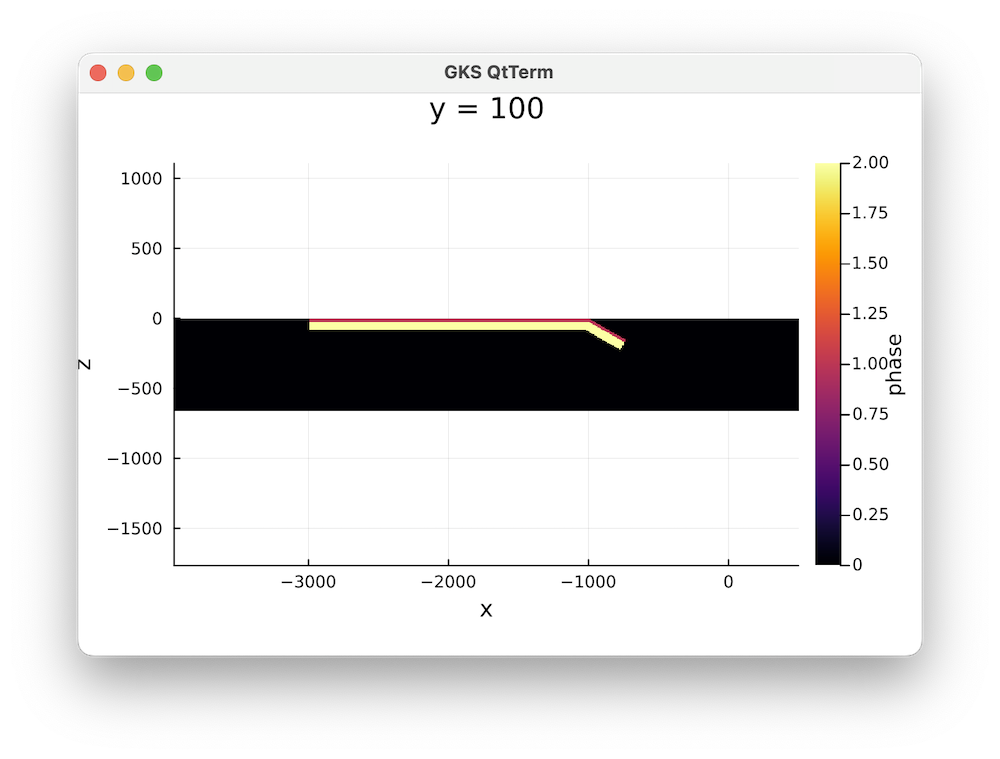

3. Add material properties:

We can specify material properties by using the Phase function

mantle = Phase(Name="mantle",ID=0,eta=1e21,rho=3200)
crust  = Phase(Name="crust", ID=1,eta=1e21,rho=3280)
slab   = Phase(Name="slab",  ID=2,eta=2e23,rho=3280)

and we can add them to the model with:

add_phase!(model, mantle, slab, crust)

You can check that this is set with:

model

LaMEM Model setup
|
|-- Scaling             :  GeoParams.Units.GeoUnits{GEO}
|-- Grid                :  nel=(128, 32, 64); xϵ(-3960.0, 500.0), yϵ(0.0, 2640.0), zϵ(-660.0, 0.0)
|-- Time                :  nstep_max=200; nstep_out=5; time_end=100.0; dt=0.05
|-- Boundary conditions :  noslip=[0, 0, 0, 0, 1, 0]
|-- Solution parameters :  eta_min=1.0e18; eta_max=1.0e25; eta_ref=1.0e20; act_temp_diff=0
|-- Solver options      :  multigrid solver; coarse grid solver=mumps; 4 levels
|-- Model setup options :  Type=files;
|-- Output options      :  filename=Subduction_3D; pvd=1; avd=0; surf=0
|-- Materials           :  3 phases;

4. Run the model

on windows MPI + mumps currently does not work

if Sys.iswindows()
    model.Solver.MGCoarseSolver = "direct"
end

Add this stage, we are ready to run the simulation. On my machine it takes around 4 seconds per timestep on 8 cores:

try testing == true

if we run this as part of the test suite, use fewer timesteps

    run_lamem(model, 8, "-nstep_max 2 -nstep_out 1")
catch
    run_lamem(model, 8)       # run on 8 cores (if possible)
end

The results looks like this with paraview: 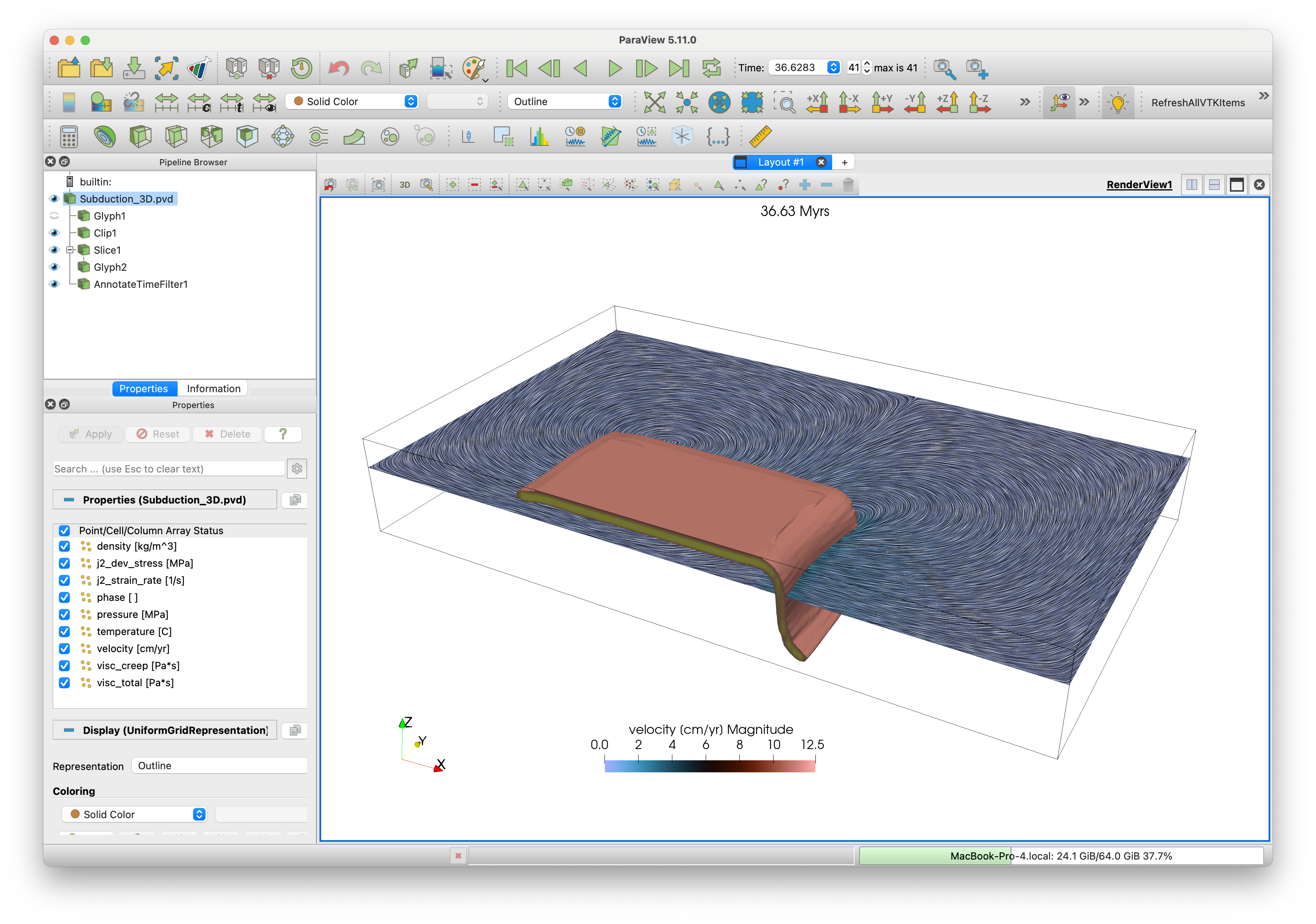Note that this is a significantly higher resolution than the original paper, which was run on an HPC system (admittedly, this was 20 years ago).

The file Subduction_3D.jl in /scripts reproduces this example

Markdown page generation

#This file was generated using Literate:
#Literate.markdown("Subduction3D.jl","../docs/src/",keepcomments=true, execute=false, codefence = "```julia" => "```")

This page was generated using Literate.jl.