Particles

Memory layout

Particles and MarkerChain store coordinates in CellArrays from CellArrays.jl. Entries are grouped by parent cell so that interpolation, advection, and reinjection routines work on spatially local chunks of memory.

Particle objects

JustPIC exposes three concrete AbstractParticles containers:

• Particles: the main cell-sorted container used for PIC workflows.

• PassiveMarkers: lightweight tracers stored as flat coordinate arrays.

• MarkerChain: a 2D interface-tracking container for free surfaces and similar boundaries.

Particles stores coordinates, active-slot masks, occupancy thresholds, and the derived center, vertex, and velocity grids used by the high-level APIs. Those extra fields are what let helpers such as move_particles!, grid2particle!, particle2grid!, inject_particles!, update_phase_ratios!, and subgrid_diffusion! use the compact (..., particles, ...) call style.

particles.np is the initial storage capacity (max_xcell * number of cells), not a live-particle count. Reduce the occupancy mask when a live count is needed.

Initialization

init_particles accepts either:

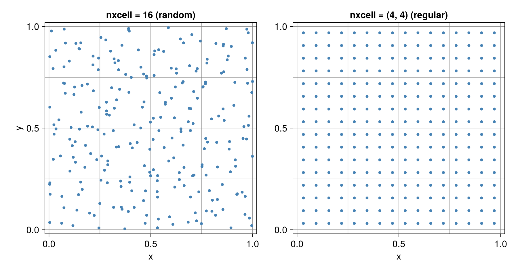
• a scalar nxcell for random, quadrant-balanced seeding inside each cell, or

• a tuple nxcell for a regular per-dimension layout, where nxcell[d] particles are placed at the centers of a uniform sub-grid of spacing dx[d] / nxcell[d] along dimension d.

If max_xcell is smaller than the resulting number of particles per cell, it is raised to match.

After construction, the returned Particles object already contains the center, vertex, and staggered velocity grids needed by the higher-level APIs.

Particle center and vertex grids use periodic ghost spacing by default. Pass a periodic tuple to init_particles for nonperiodic dimensions, such as periodic = (false, false) in 2D. Nonperiodic center ghosts reflect across the boundary vertices, using the local boundary-cell width.

The two layouts on a 4x4 grid with 16 particles per cell:

Randomly distributed particles

using JustPIC
backend   = JustPIC.CPU # device backend
nxcell    = 24  # initial number of randomly distributed particles
max_xcell = 48  # maximum number of particles per cell
min_xcell = 12  # minimum number of particles per cell
n         = 32  # number of vertices per dimension
Lx   = Ly = 1.0 # domain size
xvi       = xv, yv = LinRange(0, Lx, n), LinRange(0, Ly, n) # nodal vertices
dxi       = dx, dy = xv[2] - xv[1], yv[2] - yv[1]
xci       = xc, yc = LinRange(dx / 2, Lx - dx / 2, n - 1), LinRange(dy / 2, Ly - dy / 2, n - 1)
grid_vx   = xv, LinRange(first(yc) - dy, last(yc) + dy, length(yc) + 2)
grid_vy   = LinRange(first(xc) - dx, last(xc) + dx, length(xc) + 2), yv
## initialize particles object with randomly distributed coordinates
particles = init_particles(
    backend, nxcell, max_xcell, min_xcell, grid_vx, grid_vy,
)
sum(particles.index.data) # number of active particles

# output

23064

Regularly spaced particles

using JustPIC
backend   = JustPIC.CPU # device backend
nxcell    = (5, 5)  # number of evenly spaced particles in each cell dimension
max_xcell = 48      # maximum number of particles per cell
min_xcell = 12      # minimum number of particles per cell
n         = 32      # number of vertices per dimension
Lx   = Ly = 1.0     # domain size
xvi       = xv, yv = LinRange(0, Lx, n), LinRange(0, Ly, n) # nodal vertices
dxi       = dx, dy = xv[2] - xv[1], yv[2] - yv[1]
xci       = xc, yc = LinRange(dx / 2, Lx - dx / 2, n - 1), LinRange(dy / 2, Ly - dy / 2, n - 1)
grid_vx   = xv, LinRange(first(yc) - dy, last(yc) + dy, length(yc) + 2)
grid_vy   = LinRange(first(xc) - dx, last(xc) + dx, length(xc) + 2), yv
## initialize particles object with regularly distributed coordinates
particles = init_particles(
    backend, nxcell, max_xcell, min_xcell, grid_vx, grid_vy,
)
sum(particles.index.data) # number of active particles

# output

24025

Particle maintenance

These helpers keep the cell-sorted storage healthy as particles move: move_particles!, inject_particles!, inject_particles_phase!, clean_particles!, force_injection!, cell_index, and cell_length.

Once particles has been initialized, most transfer and maintenance routines use the geometry stored in the container directly:

grid2particle!(Fp, F, particles)
particle2grid!(F, Fp, particles)
move_particles!(particles, particle_args)
inject_particles!(particles, particle_args)
update_phase_ratios!(phase_ratios, particles, phases)

This is the preferred high-level style for simulation code, tests, and examples.

API

Containers

JustPIC.Particles Type

Particles{Backend, N, I, T1, T2, D, V} <: AbstractParticles

Main particle container used by JustPIC for material points stored cell-by-cell in CellArrays.

coords is an N-tuple of particle-coordinate arrays, index marks which slots are active inside each cell, nxcell is the target initial occupancy per cell, and min_xcell/max_xcell define the occupancy range used by injection and cleanup routines.

Use init_particles to construct this type instead of calling the inner constructor directly.

source

JustPIC.PassiveMarkers Type

PassiveMarkers{Backend,T} <: AbstractParticles

Lightweight particle container for passive tracers that only store coordinates.

Unlike Particles, passive markers do not keep per-cell occupancy metadata and are intended for tracer-style advection and interpolation workflows where the markers do not feed back into the simulation.

Use init_passive_markers to construct this type.

source

Initialization

JustPIC.init_particles Function

init_particles(backend, nxcell, max_xcell, min_xcell, grid_vx, grid_vy[, grid_vz])

Initialize a Particles container from the staggered velocity grids.

Each velocity component is supplied as an N-tuple of coordinate vectors. The diagonal coordinate vector of each component defines the particle vertex grid; the off-diagonal vectors define the cell-center grid. For example, in 2D pass grid_vx = (xv, yc_extended) and grid_vy = (xc_extended, yv).

If nxcell is a number, particles are distributed randomly within cell quadrants; the count is rounded up to a multiple of the number of quadrants so that every quadrant holds the same number of particles. If it is an NTuple, it gives the number of particles placed along each coordinate direction of every cell: nxcell[d] particles sit at the centers of a uniform sub-grid of spacing dx[d] / nxcell[d], so no particle lands on a cell boundary and the spacing is uniform across the whole domain when the grid is.

In both cases max_xcell is raised to the resulting number of particles per cell if it is smaller.

The particle vertex and center grids stored in the returned container are extended with ghost nodes. By default, ghost nodes use periodic spacing. Set periodic to false in nonperiodic dimensions to extend each boundary using its local edge spacing. The staggered velocity grids are stored as provided.

Arguments

• backend: KernelAbstractions backend type such as CPU.

• nxcell: either the target number of particles per cell, or an NTuple describing a structured per-dimension layout.

• max_xcell: number of particle slots reserved per cell.

• min_xcell: minimum occupancy used by reinjection routines.

• grid_vx, grid_vy, grid_vz: staggered velocity-grid coordinate tuples. Omit grid_vz for a 2D simulation. Each tuple must contain one coordinate vector per spatial dimension. Coordinate vectors may live on any backend; they are copied to the host to build the grids.

• periodic: tuple of booleans indicating periodic dimensions. Defaults to true in every dimension for compatibility.

Returns

• A Particles object whose coordinates and occupancy arrays are ready for advection/interpolation routines, with particles.xvi and particles.xci including one ghost node on each side.

Example

xv, yv = LinRange(0, 1, 33), LinRange(0, 1, 33)
dx = xv[2] - xv[1]
xc = LinRange(dx / 2, 1 - dx / 2, 32)
yc = xc
grid_vx = xv, LinRange(first(yc) - dx, last(yc) + dx, 34)
grid_vy = LinRange(first(xc) - dx, last(xc) + dx, 34), yv
particles = init_particles(CPU, 24, 48, 12, grid_vx, grid_vy)

# Nonperiodic boundaries on both axes
particles = init_particles(CPU, 24, 48, 12, grid_vx, grid_vy; periodic = (false, false))

# 5x5 regularly spaced particles per cell
particles = init_particles(CPU, (5, 5), 48, 12, grid_vx, grid_vy)

source

JustPIC.init_passive_markers Function

init_passive_markers(backend, coords::NTuple{N,AbstractArray})

Construct a PassiveMarkers container on backend from marker coordinate arrays.

coords is an N-tuple of vectors, one per spatial dimension, holding the initial marker positions: marker k sits at (coords[1][k], …, coords[N][k]).

Arguments

• backend: KernelAbstractions backend type such as CPU.

• coords: tuple of coordinate vectors, one per dimension.

source

JustPIC.init_cell_arrays Function

init_cell_arrays(particles::Particles, ::Val{N})

Allocate N cell-aligned scratch arrays with the same cell layout as particles.coords.

This is mainly used internally to create per-particle temporary storage for quantities such as interpolated fields or time-integration work arrays.

Returns

• An N-tuple of CellArrays with the same particle-cell layout as particles.coords.

source

Advection

JustPIC.AbstractAdvectionIntegrator Type

AbstractAdvectionIntegrator

Abstract supertype for time integrators used by particle, passive-marker, and marker-chain advection routines.

source

JustPIC.Euler Type

Euler()

Forward-Euler advection integrator.

This is the cheapest available integrator and is mainly useful for simple tests or when first-order accuracy is sufficient.

source

JustPIC.RungeKutta2 Type

RungeKutta2(α = 0.5)

Second-order Runge-Kutta advection integrator.

The parameter α controls the intermediate stage location and must satisfy 0 < α < 1. The default α = 0.5 corresponds to the midpoint method.

source

JustPIC.RungeKutta4 Type

RungeKutta4()

Classical fourth-order Runge-Kutta advection integrator.

source

JustPIC.set_precision Function

set_precision(integrator, T)

Recast an integrator's stored parameters to the scalar precision T.

This is applied at the advection launch sites so that a Float32 backend (such as Metal, which has no Float64) never carries a Float64 field into a GPU kernel. It is the identity for parameter-free integrators and, on the Float64 CPU/CUDA/AMDGPU path, a no-op (the value is preserved).

source

JustPIC.advection! Function

advection!(particles::Particles, method::AbstractAdvectionIntegrator, V, dt)
advection!(particles::Particles, method::AbstractAdvectionIntegrator, V, grid_vi, dt, dxi)

Advect particles through the staggered velocity field V over a time step dt. The particle coordinates are updated in place.

The public form reads the staggered velocity coordinate grids and spacing from particles (particles.xi_vel and particles.di.velocity), so only V and dt are supplied. The lower-level form takes those grids explicitly.

Arguments

• particles: Particles container to advect.

• method: time integrator such as Euler(), RungeKutta2(), or RungeKutta4().

• V: tuple of staggered velocity component arrays.

• dt: timestep.

• grid_vi: tuple of coordinate tuples matching the staggering of V (lower-level form only).

• dxi: grid spacing associated with grid_vi (lower-level form only).

• periodic_1, periodic_2, periodic_3: enable periodic wrapping at every integration stage in the corresponding coordinate direction.

Notes

• Use the same periodic keywords in the subsequent move_particles! call.

• Stage-wise wrapping is required by RungeKutta2 and RungeKutta4, whose intermediate interpolation points may cross a periodic boundary.

source

advection!(chain::MarkerChain, method, V, grid_vi, dt)

Advect the marker coordinates in chain through the staggered velocity field V without performing resampling or topography reconstruction.

This lower-level method is useful if you want to customize the post-advection marker-chain processing yourself.

source

advection!(particles::PassiveMarkers, method::AbstractAdvectionIntegrator, V, grid_vxi, dt)

Advect passive marker coordinates through the staggered velocity field V over a time step dt. The marker coordinates are updated in place.

Unlike the Particles method, grid_vxi must be supplied explicitly, since PassiveMarkers stores only marker coordinates and no grid metadata.

Arguments

• particles: PassiveMarkers container to advect.

• method: time integrator such as Euler(), RungeKutta2(), or RungeKutta4().

• V: tuple of staggered velocity component arrays.

• grid_vxi: tuple of coordinate tuples matching the staggering of V.

• dt: timestep.

source

JustPIC.advection_LinP! Function

advection_LinP!(particles, method, V, dt; periodic_1=false, periodic_2=false, periodic_3=false)

Advect particles using the linear-plus-pressure (LinP) velocity interpolation scheme.

This variant uses the same time integrators as advection! but evaluates velocities with the LinP reconstruction near staggered pressure points.

This method is useful when you want the interpolation behavior described in the velocity-interpolation documentation under LinP.

Periodic keywords have the same meaning as in advection! and must also be passed to the subsequent move_particles! call.

source

JustPIC.advection_MQS! Function

advection_MQS!(particles, method, V, dt; periodic_1=false, periodic_2=false, periodic_3=false)

Advect particles using the monotonic quadratic spline (MQS) velocity interpolation scheme.

Compared with advection!, this method reconstructs staggered velocities with MQS where enough stencil support is available.

Near boundaries or when the required stencil is unavailable, the implementation falls back to linear interpolation.

The public entry point reads the staggered velocity coordinates and spacing from particles.xi_vel and particles.di.velocity.

Periodic keywords have the same meaning as in advection! and must also be passed to the subsequent move_particles! call.

source

JustPIC.semilagrangian_advection! Function

semilagrangian_advection!(F, F0, method, V, grid_vi, grid, dt)

Advect a grid field with a semi-Lagrangian backtracking step.

Each destination node in F is traced backward through the velocity field V, then sampled from F0 on the vertex grid grid. grid_vi contains the staggered coordinates associated with the velocity components.

Notes

• F is overwritten in place at the interior nodes; boundary nodes are left untouched.

• F0 is the source field from the previous step and is only read.

• F and F0 must not share memory, otherwise nodes read values already overwritten by their neighbours. Aliased buffers throw an ArgumentError; pass a separate copy of the previous step instead.

• For tuple-valued fields, each component is backtracked independently.

source

semilagrangian_advection!(chain::MarkerChain, method, V, grid_vxi, grid, dt)

Advance only the vertex topography chain.h_vertices by one semi-Lagrangian step.

Each new vertex height is interpolated from forward-advected surface vertices through V (method must be RungeKutta2 or RungeKutta4, not Euler). This is the raw update used by semilagrangian_advection_markerchain!; it does not apply slope limiting, mass conservation, or marker reconstruction — call the wrapper unless you need to compose those steps yourself. Queries outside the advected horizontal chain domain sample the nearest advected endpoint height; velocity interpolation extrapolates from edge cells. The advected surface is piecewise linear, so RK order describes trajectory integration, not the spatial interpolation order. Non-finite trajectories or crossed vertices throw an error without changing the chain.

source

JustPIC.semilagrangian_advection_LinP! Function

semilagrangian_advection_LinP!(F, F0, method, V, grid_vi, grid, dt)

Semi-Lagrangian advection variant that evaluates backtracked velocities with the LinP interpolation scheme.

Use this when the advecting velocity should be reconstructed with the LinP scheme instead of plain linear interpolation.

Notes

• F is overwritten in place at the interior nodes; boundary nodes are left untouched.

• F0 is the source field from the previous step and is only read.

• F and F0 must not share memory; aliased buffers throw an ArgumentError. See semilagrangian_advection!.

source

JustPIC.semilagrangian_advection_MQS! Function

semilagrangian_advection_MQS!(F, F0, method, V, grid_vi, grid, dt)

Semi-Lagrangian advection variant that evaluates backtracked velocities with the MQS interpolation scheme.

Use this when the advecting velocity should be reconstructed with the MQS scheme instead of plain linear interpolation.

Notes

• F is overwritten in place at the interior nodes; boundary nodes are left untouched.

• F0 is the source field from the previous step and is only read.

• F and F0 must not share memory; aliased buffers throw an ArgumentError. See semilagrangian_advection!.

source

Maintenance

move_particles! drops particles whose destination cell is still full once no particle can move any more; pass verbose=true to print the number dropped. Overflow removes the particle and its companion fields together. clean_particles! removes active particles outside their stored cell; it does not compact slots. Injection with companion fields requires a live neighboring particle from which to copy field values. If that support is absent, the candidate is skipped rather than initialized with synthetic field data.

JustPIC.move_particles! Function

move_particles!(particles::AbstractParticles, args; periodic_1=false, periodic_2=false, periodic_3=false)
move_particles!(particles::AbstractParticles, grid, args, dxi; periodic_1=false, periodic_2=false, periodic_3=false)

Reassign particles to the correct parent cells after their coordinates have been updated.

This routine keeps the coordinate arrays in particles and the companion fields in args sorted by parent cell, preserving the package's spatially local memory layout.

Arguments

• particles: particle container whose coordinates have already been modified.

• args: tuple of per-particle fields that must move together with the particle coordinates.

• grid: optional vertex grid coordinates used by the lower-level method.

• dxi: optional grid spacing used by the lower-level method.

• periodic_1, periodic_2, periodic_3: enable periodic wrapping in the corresponding coordinate direction.

Notes

• Particles that leave a non-periodic direction are discarded.

• Periodic directions use the ghost cells created by add_periodic_ghost_nodes to wrap coordinates and particle fields across opposite domain boundaries. The ghost cells of a periodic direction must be empty on entry, as they are after every call; otherwise an ArgumentError is thrown.

• A particle may cross any number of cells in one call, across periodic seams included. Jumps of more than one cell make the call slower: the cells are then transferred in (2j₁ + 1) × … × (2jₙ + 1) concurrent batches, with jᵢ the largest jump along direction i, so keep the displacement per step small.

• args must use the same cell layout as particles.coords.

• The public entry point uses the vertex grid and spacing stored in particles.

• A particle whose destination cell is full stays in its source cell until the destination's own outgoing particles have left. It is dropped only once no particle can move any more, so particles exchanged between two full cells are dropped. With verbose=true, the number of dropped particles is printed. Companion fields are dropped with the particle.

source

move_particles!(chain::MarkerChain)

Reassign markers to the correct columns of chain after their coordinates have been updated.

Markers that crossed column boundaries are moved into their destination column's slots, keeping the coordinate arrays consistent with the per-column occupancy mask. A marker may cross any number of columns in one call. Markers whose updated coordinates are not finite, or which left the horizontal extent of chain.cell_vertices, are deleted.

If a destination column is full, the marker is dropped. With verbose=true, the number of such overflows is printed.

source

JustPIC.inject_particles! Function

inject_particles!(particles, args)
inject_particles!(particles, args, fields; scheme = :grid)

Inject particles into cells whose occupancy falls below particles.min_xcell.

New particles are placed quadrant by quadrant. Donors are the particles live when the call starts; particles injected by the same call are never read.

• Without fields, each entry of args is copied from the nearest donor in the 3^N cell neighborhood; a candidate with no donor is skipped.

• With fields (one grid field per entry of args, laid out as described in inject_particles_phase!), values come from scheme:

  • :grid: interpolation of fields at the new particle;

  • :least_squares: a linear least-squares fit on donors in the new particle's cell (or its 3^N neighborhood when the cell has fewer than N + 1 usable donors), clamped to the range of donor values in the neighborhood; falls back to :grid when no fit is possible.

source

JustPIC.inject_particles_phase! Function

inject_particles_phase!(particles, particles_phases, args, fields; scheme = :grid)

Phase-aware variant of inject_particles!: each new particle also copies its phase from the nearest donor. scheme selects how args are initialized, as in inject_particles!.

Each entry of fields may independently use cell centers or vertices, with one ghost sample per side on any axis or with no ghosts. Its size determines the layout relative to the particle grid. Unghosted center fields use the nearest valid interpolation stencil at boundaries, with the interpolated value clamped to the stencil's range.

source

JustPIC.clean_particles! Function

clean_particles!(particles, grid, args)

Remove active particles that no longer lie in their stored cell and keep particle-associated fields in args consistent with the particle storage layout. This routine does not compact the remaining slots.

This is typically used after particle deletion or reinjection to compact each cell's active particle block.

source

JustPIC.force_injection! Function

force_injection!(particles, p_new, fields, values)

Insert particles from p_new directly into free particle slots.

Arguments

• particles: destination Particles container.

• p_new: slot-aligned per-cell collection of coordinates to inject, with shape size(particles.index)..., cellnum(particles.index); NaN marks empty input slots.

• fields: tuple of particle fields to initialize together with the coordinates.

• values: values written into each corresponding entry of fields.

Notes

• This is a low-level routine: it does not search for nearest-neighbor values.

• Injection only happens into currently inactive particle slots.

source

force_injection!(particles, p_new)

Convenience method for force_injection! when no companion particle fields need to be initialized.

source

Phase ratios and subgrid diffusion

JustPIC.PhaseRatios Type

PhaseRatios{Backend,T}

Storage for phase-fraction fields sampled at multiple grid locations.

Depending on dimension, the container holds phase ratios at cell centers, vertices, staggered velocity nodes, and in 3D also at edge midpoints.

The fields store, for each location, the fractional occupancy of each material phase inferred from particle labels.

source

JustPIC.nphases Function

nphases(x::PhaseRatios)

Return the number of phases in x::PhaseRatios.

This method returns a Val wrapper for the phase count; use numphases when you need the integer directly.

source

JustPIC.subgrid_diffusion! Function

subgrid_diffusion!(pT, T_grid, ΔT_grid, subgrid_arrays, particles, dt; d = 1.0)

Apply the vertex-based subgrid diffusion correction to particle temperatures.

Temperatures are interpolated from the grid to particles, relaxed using the local subgrid model, mapped back to the grid as a correction, and then reapplied to the particle temperatures.

Arguments

• pT: particle temperature field updated in place.

• T_grid: source temperature on the ghosted vertex grid, sized as length.(particles.xvi).

• ΔT_grid: resolved-grid temperature increment carrying one ghost node per side, sized ncells .+ 2.

• subgrid_arrays: scratch storage created with SubgridDiffusionCellArrays(particles).

• particles: particle container.

• dt: timestep.

• d: dimensionless subgrid diffusion coefficient.

source

JustPIC.subgrid_diffusion_centroid! Function

subgrid_diffusion_centroid!(pT, T_grid, ΔT_grid, subgrid_arrays, particles, dt; d = 1.0)

Centroid-grid variant of subgrid_diffusion!.

Use this when the resolved temperature field lives at cell centers instead of vertices. T_grid is then the ghosted centroid field sized as length.(particles.xci), while ΔT_grid keeps the same ncells .+ 2 layout as in subgrid_diffusion!.

source

JustPIC.SubgridDiffusionCellArrays Type

SubgridDiffusionCellArrays(particles; loc = :vertex)

Allocate scratch storage used by the subgrid thermal diffusion routines.

The returned object stores old particle temperatures, per-particle temperature increments, characteristic diffusion timescales, and a grid-sized accumulation buffer.

loc selects whether the accumulation buffer should match a vertex-based (:vertex) or cell-centered (:center) grid layout. Either way the buffer is ghosted like particles.xvi/particles.xci.

source