Velocity interpolation
Particle and marker advection needs velocities at particle positions, while geodynamic velocity fields are usually stored on staggered grids. JustPIC offers three interpolation paths for this step.
Linear
The default advection! path uses bilinear interpolation in 2D and trilinear interpolation in 3D. This is the cheapest and most general option, and it is the right default for most examples and tests.
LinP
advection_LinP! uses the linear-plus-pressure interpolation described by Pusok et al. 2017. The velocity at the m-th particle is given by
\[u_m = A u_L + (1-A) u_P\]
where $u_L$ is the bi- or trilinear interpolation from velocity nodes to the particle, $u_P$ is the interpolation from pressure nodes to the particle, and $A = 2/3$ is an empirical coefficient.
Modified Quadratic Spline
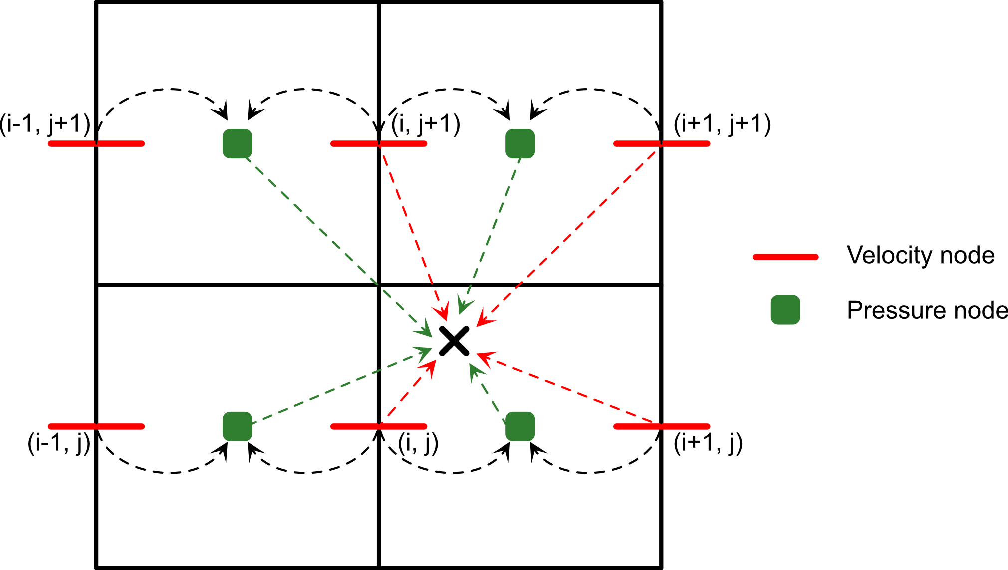
advection_MQS! uses the modified quadratic spline interpolation from Gerya et al. 2021. The scheme is designed so that velocity derivatives can be reconstructed from pressure-node locations where they are constrained by the continuity equation. Near boundaries, where the required stencil is unavailable, the implementation falls back to the linear interpolation path.
Example for the $u_x$ component in 2D:

Step 1: compute the normalized distances between the particle and the velocity node $(i, j)$ at the lower-left corner of the interpolation cell:
\[t_{x} = \frac{x_m - x_i}{\Delta x}\]
\[t_{y} = \frac{y_m - y_j}{\Delta y}\]
Step 2: lerp along $x$ on the bottom and top edges of the cell:
\[u_{m}^{\text{bot}} = (1 - t_x) u_{i,j} + t_x u_{i+1,j}\]
\[u_{m}^{\text{top}} = (1 - t_x) u_{i,j+1} + t_x u_{i+1,j+1}\]
Step 3: add the quadratic correction, a second difference along $x$ over the three nodes closest to the particle. Which triplet that is depends on which half of the cell the particle sits in — the figure above shows the $t_x < 1/2$ case:
\[u_{m}^{\text{bot}} \mathrel{+}= \frac{1}{2} \left(t_x - \frac{1}{2}\right)^2 \begin{cases} u_{i-1,j} - 2 u_{i,j} + u_{i+1,j} & t_x < 1/2 \\ u_{i,j} - 2 u_{i+1,j} + u_{i+2,j} & t_x \geq 1/2 \end{cases}\]
\[u_{m}^{\text{top}} \mathrel{+}= \frac{1}{2} \left(t_x - \frac{1}{2}\right)^2 \begin{cases} u_{i-1,j+1} - 2 u_{i,j+1} + u_{i+1,j+1} & t_x < 1/2 \\ u_{i,j+1} - 2 u_{i+1,j+1} + u_{i+2,j+1} & t_x \geq 1/2 \end{cases}\]
Step 4: lerp the corrected values along $y$:
\[u_{m} = (1-t_y) u_{m}^{\text{bot}} + t_y u_{m}^{\text{top}}\]
The $u_y$ component uses the same construction with the roles of the two directions exchanged.
Choosing a Scheme
- Use
advection!for the default linear interpolation. - Use
advection_LinP!when matching the LinP reconstruction from the cited PIC literature. - Use
advection_MQS!when the modified quadratic spline stencil is desired and the grid has enough interior support. - Use
semilagrangian_advection!,semilagrangian_advection_LinP!, orsemilagrangian_advection_MQS!for grid-field backtracking with the corresponding velocity reconstruction.