Moho Topography

Goal

This explains how to load the Moho topography for Italy and the Alps and create a paraview file. The data comes from the following publication: Spada, M., Bianchi, I., Kissling, E., Agostinetti, N.P., Wiemer, S., 2013. Combining controlled-source seismology and receiver function information to derive 3-D Moho topography for Italy. Geophysical Journal International 194, 1050–1068. doi:10.1093/gji/ggt148

1. Download data

The data is available as digital dataset on the Researchgate page of Prof. Edi Kissling https://www.researchgate.net/publication/322682919_Moho_Map_Data-WesternAlps-SpadaETAL2013

We have also uploaded it here: https://seafile.rlp.net/d/a50881f45aa34cdeb3c0/

The full data set actually includes 3 different Moho's (Europe, Adria, Tyrrhenia-Corsica). To simplify matters, we have split the full file into 3 separate ascii files and uploaded it.

We start with loading the necessary packages

using DelimitedFiles, GeophysicalModelGenerator

Please download the files

• Moho_Map_Data-WesternAlps-SpadaETAL2013_Moho1.txt

• Moho_Map_Data-WesternAlps-SpadaETAL2013_Moho2.txt

• Moho_Map_Data-WesternAlps-SpadaETAL2013_Moho3.txt.

This can be done using download_data:

download_data("https://seafile.rlp.net/d/a50881f45aa34cdeb3c0/files/?p=%2FMoho_Map_Data-WesternAlps-SpadaETAL2013_Moho1.txt&dl=1","Moho_Map_Data-WesternAlps-SpadaETAL2013_Moho1.txt")
download_data("https://seafile.rlp.net/d/a50881f45aa34cdeb3c0/files/?p=%2FMoho_Map_Data-WesternAlps-SpadaETAL2013_Moho2.txt&dl=1","Moho_Map_Data-WesternAlps-SpadaETAL2013_Moho2.txt")
download_data("https://seafile.rlp.net/d/a50881f45aa34cdeb3c0/files/?p=%2FMoho_Map_Data-WesternAlps-SpadaETAL2013_Moho3.txt&dl=1","Moho_Map_Data-WesternAlps-SpadaETAL2013_Moho3.txt")

2. Read data into Julia

The data sets start at line 39. We read this into julia as:

data            = readdlm("Moho_Map_Data-WesternAlps-SpadaETAL2013_Moho1.txt",' ',Float64,'\n', skipstart=38,header=false)
lon, lat, depth = data[:,1], data[:,2], -data[:,3];
nothing #hide

Note that depth is made negative.

3. Reformat the data

Next, let's check if the data is spaced in a regular manner in Lon/Lat direction. For that, we plot it using the Plots package (you may have to install that first on your machine).

using Plots
scatter(lon,lat,marker_z=depth, ylabel="latitude",xlabel="longitude",markersize=2.5, c = :roma)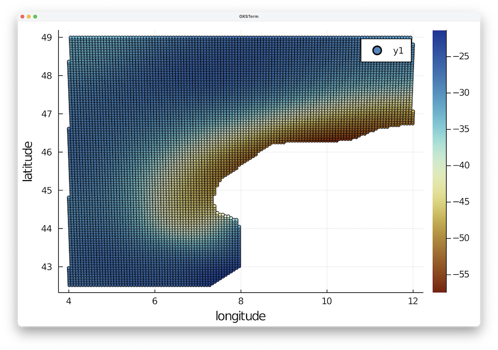

What we can see nicely here is that the data is reasonably regular but also that there are obviously locations where no data is define.

The easiest way to transfer this to Paraview is to simply save this as 3D data points:

using GeophysicalModelGenerator
data_Moho1 = GeoData(lon,lat,depth,(MohoDepth=depth*km,))

GeoData
  size  : (12355,)
  lon   ϵ [ 4.00026 - 11.99991]
  lat   ϵ [ 42.51778 - 48.99544]
  depth ϵ [ -57.46 km - -21.34 km]
  fields: (:MohoDepth,)

write_paraview(data_Moho1, "Spada_Moho_Europe", PointsData=true)

And we can do the same with the other two Moho's:

data = readdlm("Moho_Map_Data-WesternAlps-SpadaETAL2013_Moho2.txt",' ',Float64,'\n', skipstart=38,header=false);
lon, lat, depth        = data[:,1], data[:,2], -data[:,3];
data_Moho2 = GeoData(lon,lat,depth,(MohoDepth=depth*km,))
write_paraview(data_Moho2, "Spada_Moho_Adria", PointsData=true)
data =readdlm("Moho_Map_Data-WesternAlps-SpadaETAL2013_Moho3.txt",' ',Float64,'\n', skipstart=38,header=false);
lon, lat, depth        = data[:,1], data[:,2], -data[:,3];
data_Moho3 = GeoData(lon,lat,depth,(MohoDepth=depth*km,))
write_paraview(data_Moho3, "Spada_Moho_Tyrrhenia", PointsData=true)

If we plot this in paraview, it looks like this: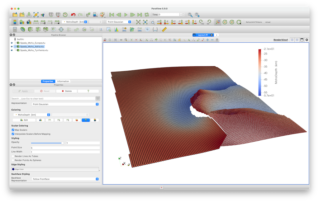

4. Fitting a mesh through the data

So obviously, the Moho is discontinuous between these three Mohos. Often, it looks nicer if we fit a regular surface through these data points. To do this we first combine the data points of the 3 surfaces into one set of points

lon   = [data_Moho1.lon.val;   data_Moho2.lon.val;   data_Moho3.lon.val];
lat   = [data_Moho1.lat.val;   data_Moho2.lat.val;   data_Moho3.lat.val];
depth = [data_Moho1.depth.val; data_Moho2.depth.val; data_Moho3.depth.val];
data_Moho_combined = GeoData(lon, lat, depth, (MohoDepth=depth*km,))

Next, we define a regular lon/lat grid

Lon, Lat, Depth  = lonlatdepth_grid(4.1:0.1:11.9,42.5:.1:49,-30km)

We will use a nearest neighbor interpolation method to fit a surface through the data, which has the advantage that it will take the discontinuities into account. This can be done with nearest_point_indices

idx = nearest_point_indices(Lon,Lat, lon[:],lat[:])
Depth = depth[idx]

Now, we can create a GeoData structure with the regular surface and save it to paraview:

data_Moho = GeoData(Lon, Lat, Depth, (MohoDepth=Depth,))
write_paraview(data_Moho, "Spada_Moho_combined")

The result is shown here, where the previous points are colored white and are a bit smaller. Obviously, the datasets coincide well.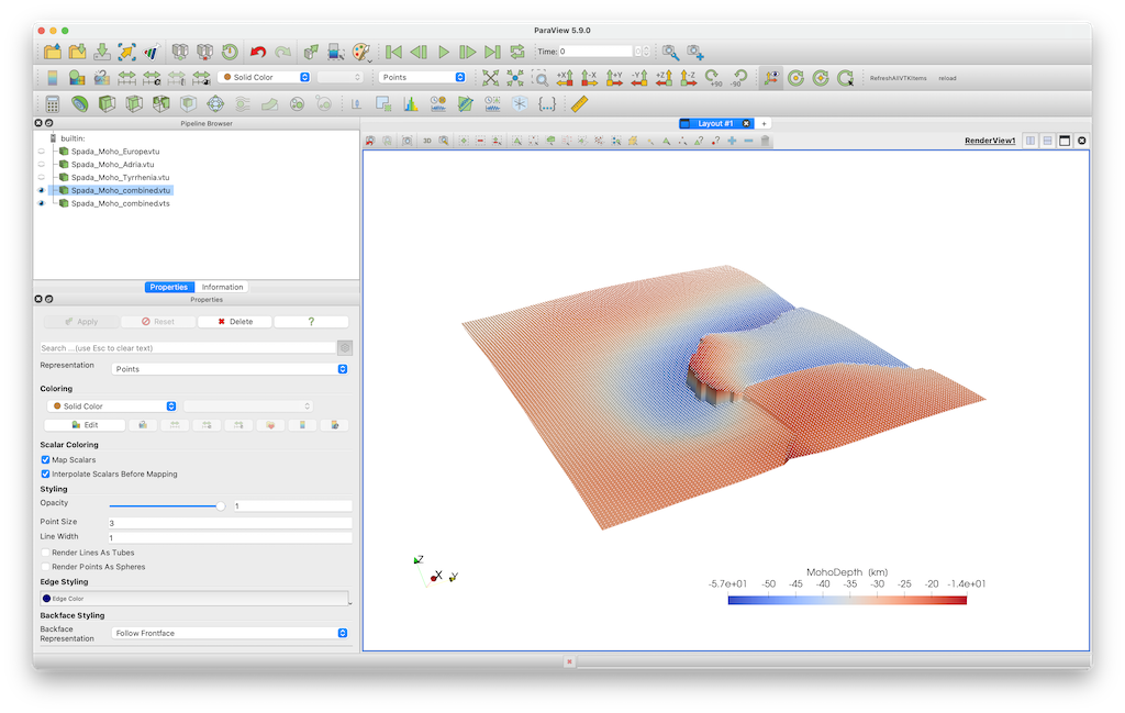

5. Julia script

The full julia script that does it all is given here.

---

This page was generated using Literate.jl.