Conductivity
Methods
Thermal conductivity is defined as
GeoParams.MaterialParameters.Conductivity.ConstantConductivity Type
ConstantConductivity(k=3.0W/m/K)Set a constant conductivity
where
GeoParams.MaterialParameters.Conductivity.T_Conductivity_Whittington Type
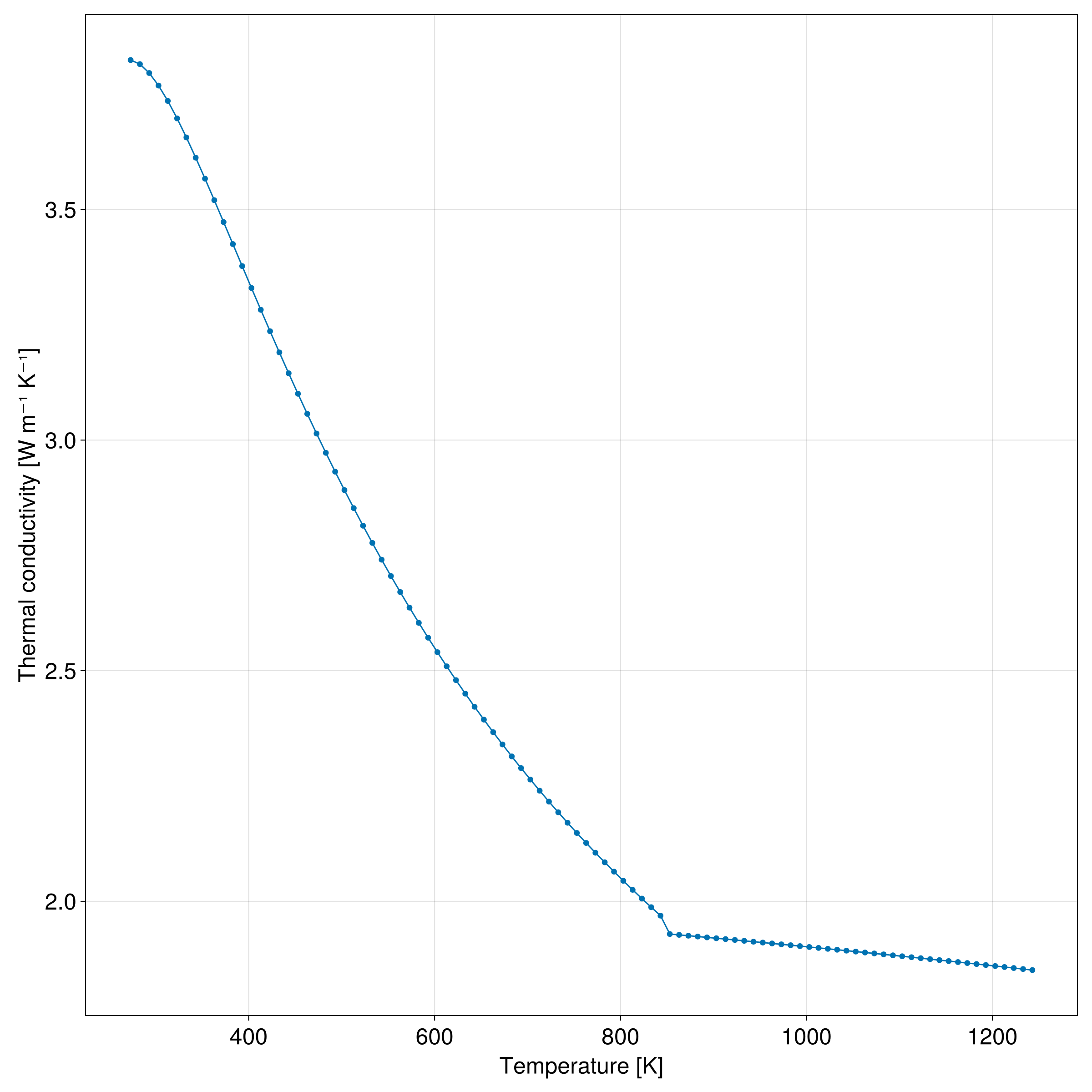
T_Conductivity_Whittington()Sets a temperature-dependent conductivity following the parameterization of _Whittington, A.G., Hofmeister, A.M., Nabelek, P.I., 2009. Temperature-dependent thermal diffusivity of the Earth’s crust and implications for magmatism. Nature 458, 319–321. https://doi.org/10.1038/nature07818._ Their parameterization is originally given for the thermal diffusivity, together with a parameterization for thermal conductivity, which allows us to compute
where T:
a = 199.50 J/mol/K if T<= 846 K
a = 199.50 J/mol/K if T> 846 K
b = 0.0857J/mol/K^2 if T<= 846 K
b = 0.0323J/mol/K^2 if T> 846 K
c = 5e6J/mol*K if T<= 846 K
c = 47.9e-6J/mol*K if T> 846 K
d = 567.3m^2/s*K
e = 0.062m^2/s
f = 0.732m^2/s
g = 0.000135m^2/s/K
This looks like:
Example
julia> using GLMakie, GeoParams
julia> p=T_Conductivity_Whittington();
julia> T,k,plt = PlotConductivity(p)GeoParams.MaterialParameters.Conductivity.T_Conductivity_Whittington_parameterised Type
T_Conductivity_Whittington_parameterised()Sets a temperature-dependent conductivity that is parameterization after Whittington, et al. 2009
The original parameterization involves quite a few parameters; this is a polynomial fit that is roughly valid from 0-1000 Celsius
where T[K] is the temperature in Kelvin (or the nondimensional equivalent of it).
The comparison of this parameterisation vs. the original one is: 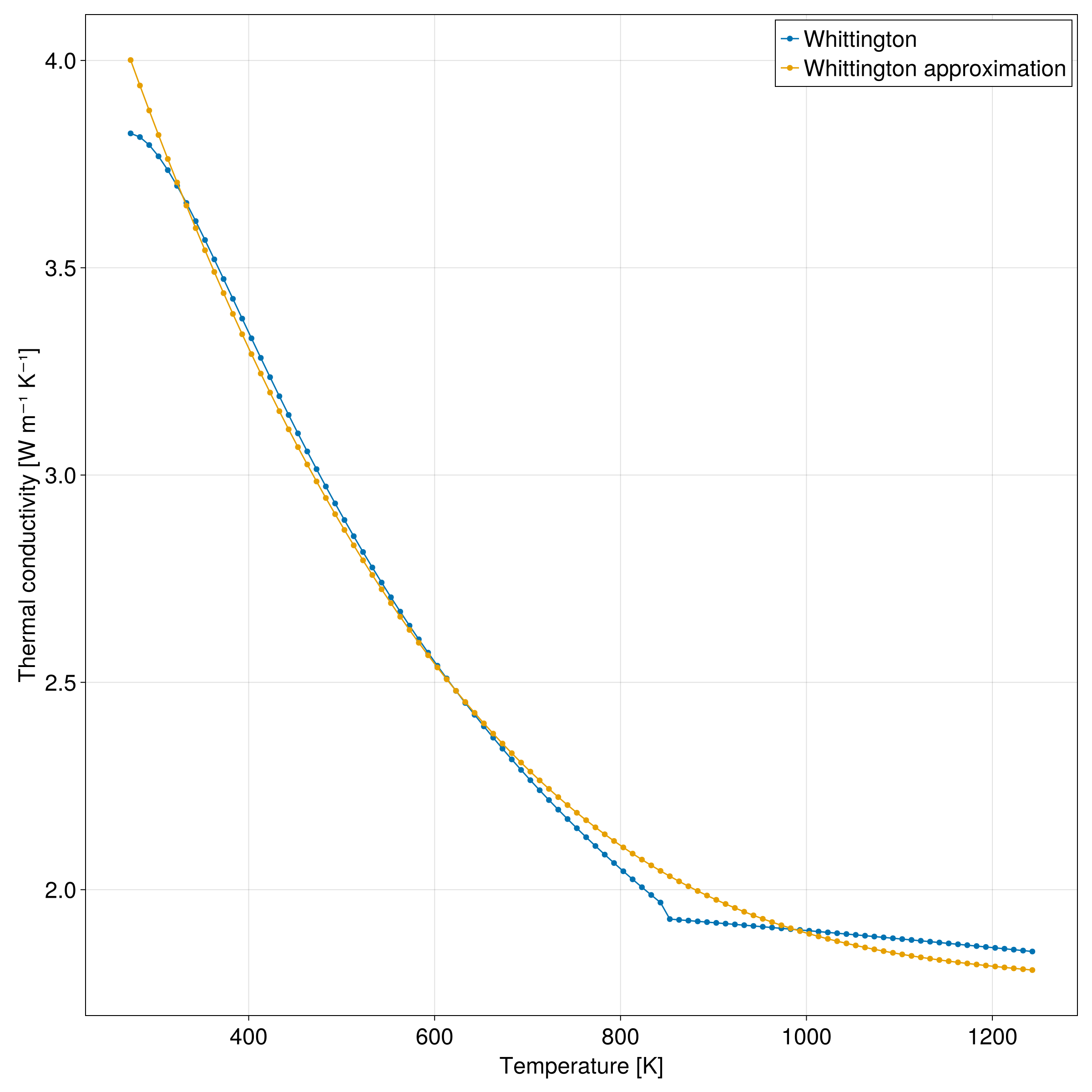
GeoParams.MaterialParameters.Conductivity.TP_Conductivity Type
TP_Conductivity()Sets a temperature (and pressure)-dependent conductivity parameterization as described in Gerya, Numerical Geodynamics (2nd edition, Table 21.2). The general for
where T and pressure P:
= 1.18Watt/K/m = 474Watt/m = 77K = 0/MPa
GeoParams.MaterialParameters.Conductivity.Set_TP_Conductivity Function
Set_TP_Conductivity(name::String)Returns the pre-defined temperature(-pressure) dependent conductivity law name.
Available laws:
"UpperCrust"
"LowerCrust"
"OceanicCrust"
"Mantle"
Example
julia> k = Set_TP_Conductivity("Mantle")
T/P dependent conductivity: Name = Mantle, k = (0.73 + 1293.0/(T + 77.0))*(1 + 4.0e-5*P)GeoParams.MaterialParameters.Conductivity.T_Conductivity_Moitra Type
T_Conductivity_Moitra(; ρ=ConstantDensity(ρ=3000kg/m^3), Cp=T_HeatCapacity_Moitra())Thermal conductivity
with
a0 = 5.98 mm²/s K^0.41, b0 = 9.23e-5 mm²/s/K
a1 = -0.06 mm²/s, b1 = 4.57e-4 mm²/s/K
Tg = 1000 K
The density ρ and heat capacity Cp are laws evaluated with the same arguments, so T_Conductivity_Moitra_smoothed replaces the jump by a smooth transition. Above 1273 K the melt branches are extrapolated. Moitra et al. (2018, p. 3627) attribute the rise of
References
- Moitra, P., Sonder, I., Valentine, G. A. (2018), Effects of size and temperature-dependent thermal conductivity on the cooling of pyroclasts in air, G-cubed 19, 3623-3636, https://doi.org/10.1029/2018GC007510
GeoParams.MaterialParameters.Conductivity.T_Conductivity_Moitra_smoothed Type
T_Conductivity_Moitra_smoothed(; ρ=ConstantDensity(ρ=3000kg/m^3), Cp=T_HeatCapacity_Moitra_smoothed())T_Conductivity_Moitra with the jump of the diffusivity at
with the glass and melt diffusivities of T_Conductivity_Moitra and the same T_HeatCapacity_Moitra_smoothed, the default Cp. The default
GeoParams.MaterialParameters.Conductivity.IAPWS_H2O_Conductivity Type
IAPWS_H2O_Conductivity(; ρ=HalbachChatterjee_Density(), L0, L1)Thermal conductivity of H2O from the IAPWS 2011 formulation (Huber et al. 2012; IAPWS R15-11, eqs. 15-17) without the critical-enhancement term
with L0 (L1 (ρ evaluated with the same arguments (P, T).
IAPWS R15-11 validates the formulation (its eq. 14) up to 1173.15 K for Tref, ρref and kref are
References
Huber, M. L., Perkins, R. A., Friend, D. G., et al. (2012), New International Formulation for the Thermal Conductivity of H2O, J. Phys. Chem. Ref. Data 41, 033102, https://doi.org/10.1063/1.4738955
IAPWS R15-11 (2011), Release on the IAPWS Formulation 2011 for the Thermal Conductivity of Ordinary Water Substance, https://iapws.org/technical-guidance/release/ThCond
GeoParams.MaterialParameters.Conductivity.GasMixture_Conductivity Type
GasMixture_Conductivity(; kh2o=IAPWS_H2O_Conductivity(), kco2=ConstantConductivity(k=0.071W/m/K))Thermal conductivity of a binary H2O-CO2 gas mixture after Udoetok (2013), eq. 16, the mean of the parallel (eq. 14) and series (eq. 9) arrangements of the two gases:
The CO2 mole fraction of the gas X_co2 is passed at runtime, as for the H2O-CO2 solubility laws; kh2o and kco2 are conductivity laws evaluated with the remaining arguments (e.g. T). The result is NaN outside kh2o depends on P and T; the default kco2 = 0.071 W/m/K is the conductivity of CO2 at 1000 K and low pressure. Over 600-1200 °C and 0.1-400 MPa the conductivity of CO2 ranges from 0.06 to 0.15 W/m/K, so the default underestimates it by up to a factor of about 2 at high pressure.
References
- Udoetok, E. S. (2013), Thermal conductivity of binary mixtures of gases, Frontiers in Heat and Mass Transfer 4, 023008, https://doi.org/10.5098/hmt.v4.2.3008
GeoParams.MaterialParameters.Conductivity.Maxwell_Conductivity Type
Maxwell_Conductivity(; kmatrix=T_Conductivity_Moitra(), kgas=GasMixture_Conductivity())Effective thermal conductivity of a matrix containing non-interacting spherical gas bubbles, the Maxwell equation used by Heap et al. (2020), eq. 1, with
where kmatrix: melt, including any crystals) and kgas). The second form, used here, stays finite at ϕ_gas is passed at runtime; both sub-laws receive the remaining arguments (e.g. P, T, X_co2; the default kgas needs P and T). kgas is only evaluated when ϕ_gas != 0. The result is NaN outside
The Maxwell equation assumes dilute, non-interacting bubbles. For kmatrix inherits the melt-branch limitation of T_Conductivity_Moitra above
References
- Heap, M. J., et al. (2020), The thermal properties of porous andesite, JVGR 398, 106901, https://doi.org/10.1016/j.jvolgeores.2020.106901
Conductivity of magma
T_Conductivity_Moitra computes T_Conductivity_Moitra_smoothed uses the same transition.
using GeoParams, CairoMakie
T = range(300, 1400, 1101)
fig = Figure(size = (800, 450))
ax = Axis(fig[1, 1]; xlabel = "temperature T (K)", ylabel = "conductivity k (W/m/K)")
vspan!(ax, 1273, 1400; color = (:gray, 0.2), label = "extrapolated (> 1273 K)")
vlines!(ax, 1000; color = :black, linestyle = :dot, label = "T_g = 1000 K")
for (name, law) in ("T_Conductivity_Moitra" => T_Conductivity_Moitra(), "T_Conductivity_Moitra_smoothed (ΔTg = 20 K)" => T_Conductivity_Moitra_smoothed())
    lines!(ax, T, [compute_conductivity(law, (; T = t)) for t in T]; label = name)
end
axislegend(ax; position = :lt)
fig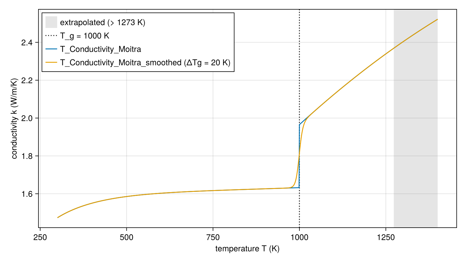
The conductivity of the gas phase: IAPWS_H2O_Conductivity is solid where IAPWS R15-11 validates the formulation and dashed where it is extrapolated. GasMixture_Conductivity mixes it with the default constant CO2 conductivity.
using GeoParams, CairoMakie
# IAPWS R15-11 validates the formulation for T ≤ 1173.15 K at P ≤ 100 MPa, T ≤ 874 K at P ≤ 250 MPa, T ≤ 573 K above
validated(P, T) = (P ≤ 1.0e8 && T ≤ 1173.15) || (P ≤ 2.5e8 && T ≤ 874.0) || T ≤ 573.0
kh2o = IAPWS_H2O_Conductivity()
P = exp10.(range(5, log10(4.0e8), 200))
fig = Figure(size = (1000, 420))
ax1 = Axis(fig[1, 1]; xscale = log10, xlabel = "pressure P (MPa)", ylabel = "k (W/m/K)", title = "IAPWS_H2O_Conductivity (dashed: extrapolated)")
for (i, Tc) in enumerate((600, 850, 1100))
    T = Tc + 273.15
    k = [compute_conductivity(kh2o, (; P = p, T)) for p in P]
    lines!(ax1, P ./ 1.0e6, k; color = Cycled(i), linestyle = :dash)
    lines!(ax1, P ./ 1.0e6, [validated(p, T) ? ki : NaN for (p, ki) in zip(P, k)]; color = Cycled(i), label = "$Tc °C")
end
axislegend(ax1; position = :lt)
ax2 = Axis(fig[1, 2]; xlabel = "CO2 mole fraction of the gas X_co2 (–)", ylabel = "k (W/m/K)", title = "GasMixture_Conductivity, 850 °C")
X = range(0, 1, 101)
for p in (1.0e7, 1.0e8, 3.0e8)
    lines!(ax2, X, [compute_conductivity(GasMixture_Conductivity(), (; P = p, T = 1123.15, X_co2 = x)) for x in X]; label = "$(round(Int, p / 1.0e6)) MPa")
end
axislegend(ax2; position = :rt)
fig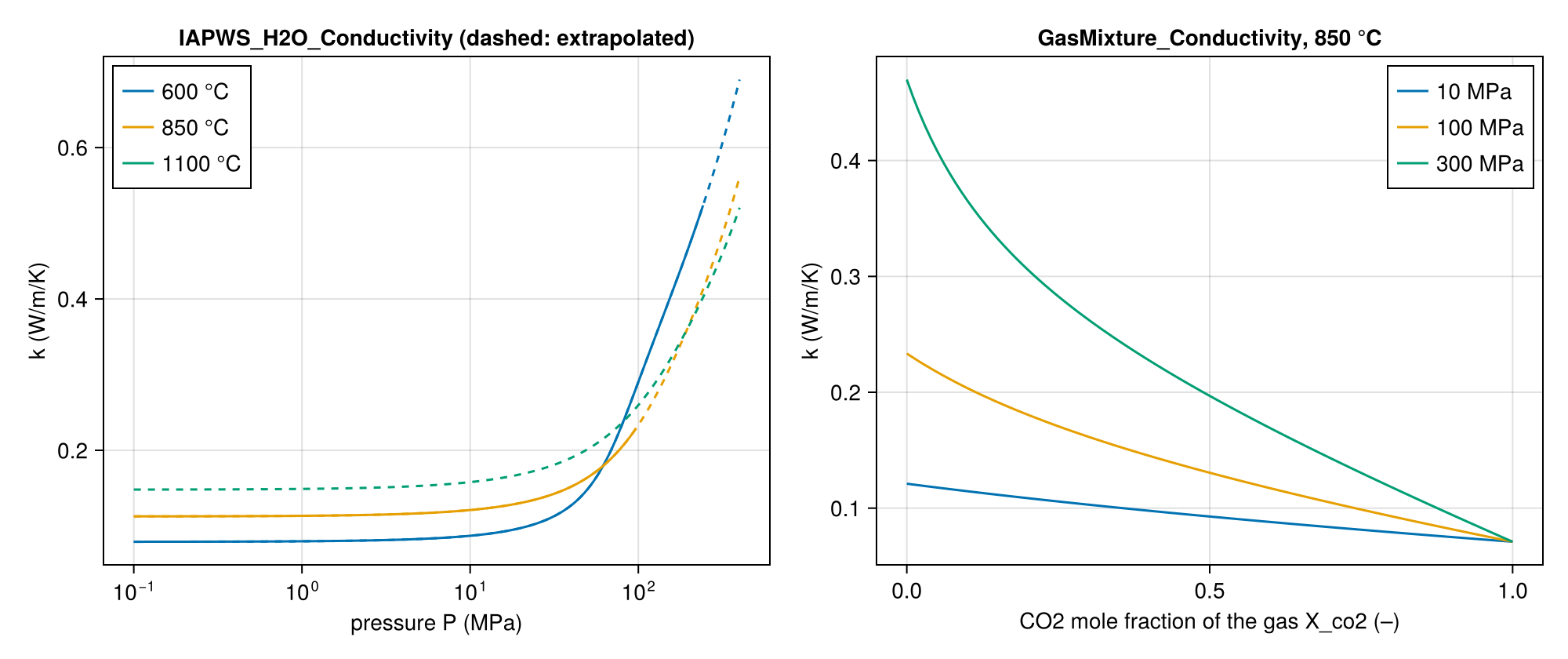
Maxwell_Conductivity combines a matrix with gas bubbles. With its defaults, a Moitra matrix and an H2O gas, the bubbles lower the magma conductivity roughly in proportion to the gas fraction.
using GeoParams, CairoMakie
k = Maxwell_Conductivity()
ϕ_gas = range(0, 0.8, 161)
fig = Figure(size = (800, 450))
ax = Axis(fig[1, 1]; xlabel = "gas fraction ϕ_gas (–)", ylabel = "conductivity k (W/m/K)", title = "Maxwell_Conductivity: Moitra matrix with H2O bubbles at 50 MPa")
for T in (900.0, 1200.0)
    lines!(ax, ϕ_gas, [compute_conductivity(k, (; P = 5.0e7, T, ϕ_gas = g)) for g in ϕ_gas]; label = "T = $(round(Int, T)) K")
end
axislegend(ax; position = :rt)
fig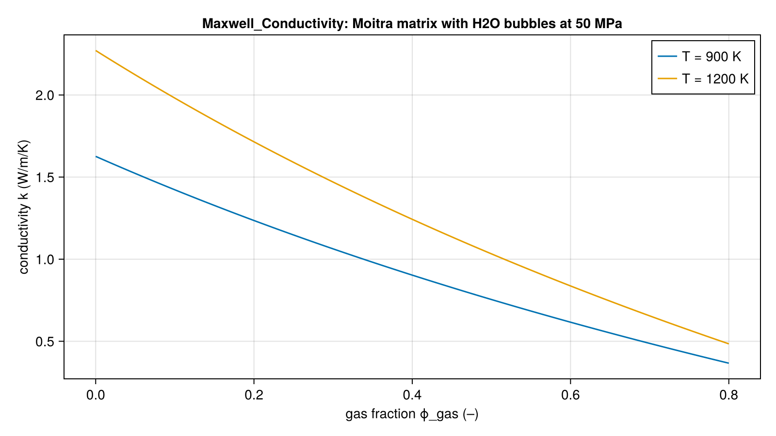
Computational routines
To compute, use this:
GeoParams.MaterialParameters.Conductivity.compute_conductivity Function
k = compute_conductivity(s::AbstractConductivity; P, T)
k = compute_conductivity(s::AbstractConductivity, args)
Returns the thermal conductivity k for the parameterization s, evaluated at the temperature T and pressure P passed either as keyword arguments or as a NamedTuple args.
Currently available:
ConstantConductivity
T_Conductivity_Whittington
TP_Conductivity
T_Conductivity_Moitra
T_Conductivity_Moitra_smoothed
IAPWS_H2O_Conductivity
GasMixture_Conductivity
Maxwell_Conductivity
Example
julia> k = T_Conductivity_Whittington();

julia> compute_conductivity(k; T = 1000.0)
1.9014576517265882GeoParams.MaterialParameters.Conductivity.compute_conductivity! Function
compute_conductivity(k_array::AbstractArray{<:AbstractFloat,N},P::AbstractArray{<:AbstractFloat,N},T::AbstractArray{<:AbstractFloat,N}, s::ConstantConductivity) where NIn-place routine to compute constant conductivity
sourcecompute_conductivity!(K::AbstractArray{<:AbstractFloat}, Phases::AbstractArray{<:Integer}, P::AbstractArray{<:AbstractFloat},Temp::AbstractArray{<:AbstractFloat}, MatParam::AbstractArray{<:AbstractMaterialParamsStruct})In-place computation of conductivity K for the whole domain and all phases, in case a vector with phase properties MatParam is provided, along with P and Temp arrays. This assumes that the Phase of every point is specified as an Integer in the Phases array.
compute_conductivity!(k::AbstractArray{T,N}, PhaseRatios::AbstractArray{T, M}, P::AbstractArray{<:AbstractFloat,N},T::AbstractArray{<:AbstractFloat,N}, MatParam::AbstractArray{<:AbstractMaterialParamsStruct})In-place computation of conductivity k for the whole domain and all phases, in case a vector with phase properties MatParam is provided, along with P and T arrays. This assumes that the PhaseRatio of every point is specified as an Integer in the PhaseRatios array, which has one dimension more than the data arrays (and has a phase fraction between 0-1)