Melting Parameterizations

Methods

A number of melting parameterisations are implemented, which can be set with:

GeoParams.MeltingParam.MeltingParam_Caricchi Type

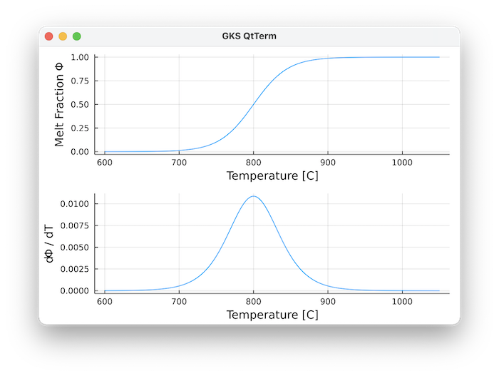
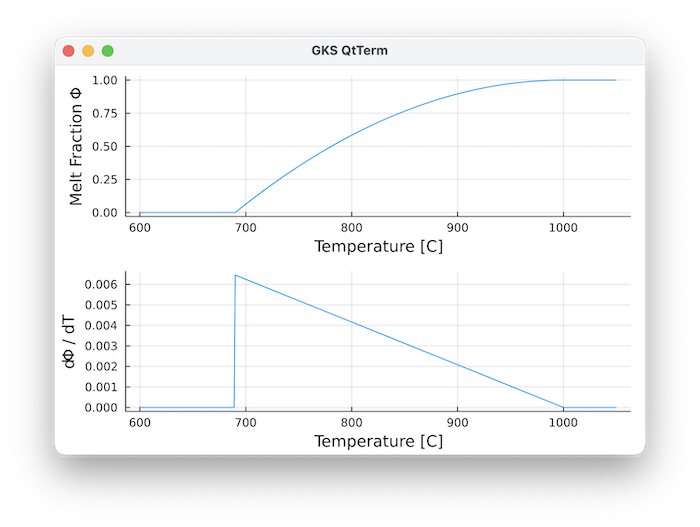
MeltingParam_Caricchi()

Implements the T-dependent melting parameterisation used by Caricchi, Simpson et al. (as for example described in Simpson)

$$\theta =\frac{a-(T+c)}{b}$$$${\varphi }_{melt}=\frac{1.0}{1.0+e^{\theta }}$$

Note that T is in Kelvin. As default parameters we employ:

$$b=23K,a=800K,c=273.15K$$

Which gives a reasonable fit to experimental data of granodioritic composition (Piwinskii and Wyllie, 1968):

References

• Simpson G. (2017) Practical finite element modelling in Earth Sciences Using MATLAB.

source

GeoParams.MeltingParam.MeltingParam_Smooth3rdOrder Type

MeltingParam_Smooth3rdOrder()

Implements the a smooth 3rd order T-dependent melting parameterisation (as used by Melnik and coworkers)

$$x=\frac{T-273.15}{1000.0}$$$$\theta =a+b\ast x+c\ast x^2+d\ast x^3$$$${\varphi }_{melt}=\frac{1.0}{1.0+e^{\theta }}$$

Note that T is in Kelvin.

As default parameters we employ:

$$a=517.9,b=-1619.0,c=1699.0,d=-597.4$$

which gives a reasonable fit to experimental data for basalt.

Data for rhyolite are:

$$a=3043.0,b=-10552.0,c=12204.9,d=-4709.0$$

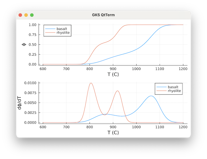Red: Rhyolite, Blue: Basalt

References

source

GeoParams.MeltingParam.MeltingParam_5thOrder Type

MeltingParam_5thOrder(a,b,c,d,e,f,T_s,T_l)

Uses a 5th order polynomial to describe the melt fraction phi between solidus temperature T_s and liquidus temperature T_l

$$\varphi =a{T}^5+b{T}^4+c{T}^3+d{T}^2+eT+f\text{ for }{T}_s\le T\le T_l$$$$\varphi =1\text{ if }T>T_l$$$$\varphi =0\text{ if }T<T_s$$

Temperature T is in Kelvin.

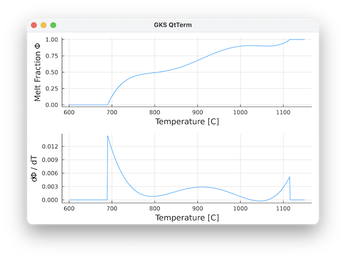
The default values are for a composite liquid-line-of-descent:

• the upper part is for Andesite from: (Blatter, D. L. & Carmichael, I. S. (2001) Hydrous phase equilibria of a Mexican highsilica andesite: a candidate for a mantle origin? Geochim. Cosmochim. Acta 65, 4043–4065

• the lower part is extrapolated to the granitic minimum using the Marxer & Ulmer LLD for Andesite (Marxer, F. & Ulmer, P. (2019) Crystallisation and zircon saturation of calc-alkaline tonalite from the Adamello Batholith at upper crustal conditions: an experimental study. Contributions Mineral. Petrol. 174, 84)

source

GeoParams.MeltingParam.MeltingParam_4thOrder Type

MeltingParam_4thOrder(b,c,d,e,f,T_s,T_l)

Uses a 4th order polynomial to describe the melt fraction phi between solidus temperature T_s and liquidus temperature T_l

$$\varphi =b{T}^4+c{T}^3+d{T}^2+eT+f\text{ for }{T}_s\le T\le T_l$$$$\varphi =1\text{ if }T>T_l$$$$\varphi =0\text{ if }T<T_s$$

Temperature T is in Kelvin.

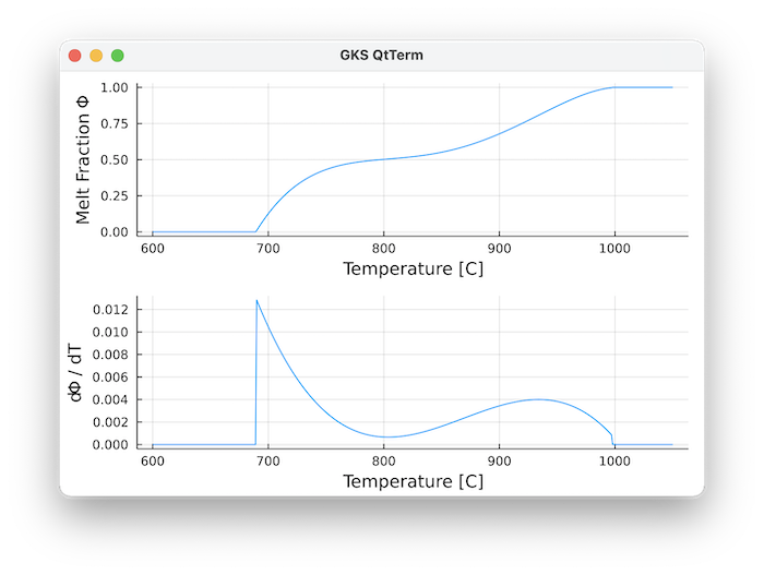
The default values are for Tonalite experiments from Marxer and Ulmer (2019):

• Marxer, F. & Ulmer, P. (2019) Crystallisation and zircon saturation of calc-alkaline tonalite from the Adamello Batholith at upper crustal conditions: an experimental study. Contributions Mineral. Petrol. 174, 84

source

GeoParams.MeltingParam.MeltingParam_Quadratic Type

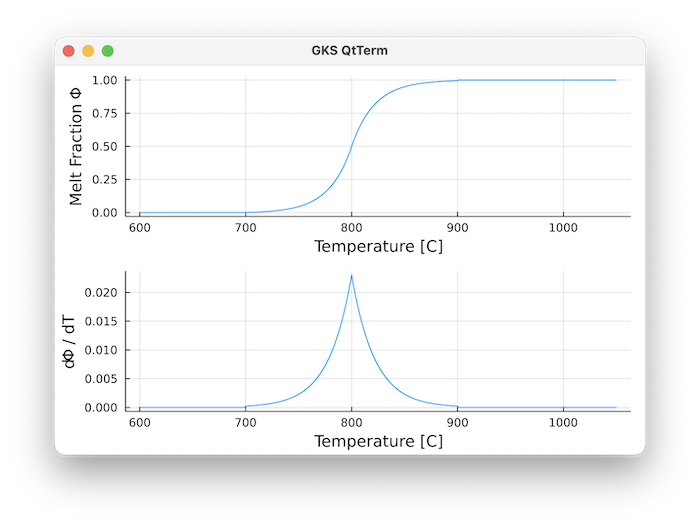
MeltingParam_Quadratic(T_s,T_l)

Quadratic melt fraction parameterisation where melt fraction $\varphi$ depends only on solidus ($T_s$) and liquidus ($T_l$) temperature:

$$\varphi =1.0-{\left(\frac{T_l-T}{T_l-T_s}\right)}^2$$$$\varphi =1.0\text{ if }T>T_l$$$$\varphi =0.0\text{ if }T<T_s$$

Temperature T is in Kelvin.

This was used, among others, in Tierney et al. (2016) Geology

source

GeoParams.MeltingParam.MeltingParam_Assimilation Type

MeltingParam_Assimilation(T_s,T_l,a)

Melt fraction parameterisation that takes the assimilation of crustal host rocks into account, as used by Tierney et al. (2016) based upon a parameterisation of Spera and Bohrson (2001)

Here, the fraction of molten and assimilated host rocks $\varphi$ depends on the solidus ($T_s$) and liquidus ($T_l$) temperatures of the rocks, as well as on a parameter $a=0.005$

$$X=\frac{T-T_s}{T_l-T_s}$$$$\varphi =a\cdot ({\exp }^{2ln(100)X}-1.0)\text{ if }X\le 0.5$$$$\varphi =1-a\cdot {\exp }^{2ln(100)(1-X)}\text{ if }X>0.5$$$$\varphi =1.0\text{ if }T>T_l$$$$\varphi =0.0\text{ if }T<T_s$$

Temperature T is in Kelvin.

This was used, among others, in Tierney et al. (2016), who employed as default parameters:

$$T_s=973.15,T_l=1173.15,a=0.005$$

References

• Spera, F.J., and Bohrson, W.A., 2001, Energy-Constrained Open-System Magmatic Processes I: General Model and Energy-Constrained Assimilation and Fractional Crystallization (EC- AFC) Formulation: Journal of Petrology, v. 42, p. 999–1018.

• Tierney, C.R., Schmitt, A.K., Lovera, O.M., de Silva, S.L., 2016. Voluminous plutonism during volcanic quiescence revealed by thermochemical modeling of zircon. Geology 44, 683–686. https://doi.org/10.1130/G37968.1

source

GeoParams.MeltingParam.SmoothMelting Type

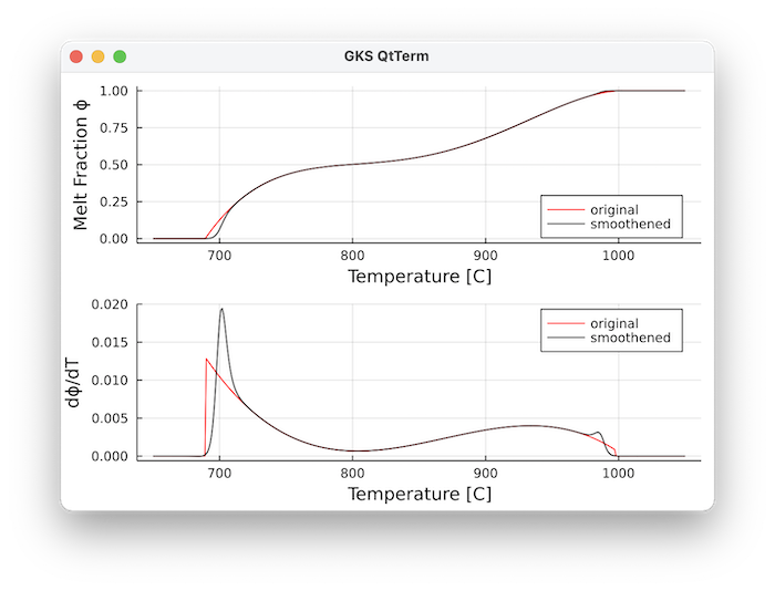
SmoothMelting(; p=MeltingParam_4thOrder(), k_sol=0.2/K,  k_liq=0.2/K)

This smoothens the melting parameterisation $p$ around the solidus $T_{sol}$ and liquidus $T_{liq}$ using a smoothened Heaviside step functions for the solidus:

$$H_{sol}=\frac{1.0}{1+\exp (-2k_{sol}(T-T_{sol}-\frac{2}{k_{sol}}))}$$

and liquidus:

$$H_{liq}=1.0-\frac{1.0}{1+\exp (-2k_{liq}(T-T_{liq}+\frac{2}{k_{liq}}))}$$

The resulting melt fraction $\varphi$ is computed from the original melt fraction ${\varphi }_0$ (computed using one of the methods above) as:

$$\varphi ={\varphi }_0{H}_{sol}{H}_{liq}+1.0-H_{liq}$$

The width of the smoothening zones is controlled by $k_{sol},k_{liq}$ (larger values = sharper boundary).

This is important, as jumps in the derivative $d\varphi /dT$ can cause numerical instabilities in latent heat computations, which is prevented with this smoothening.

Example

Let's consider a 4th order parameterisation:

julia> using GLMakie, GeoParams
julia> p = MeltingParam_4thOrder();
julia> T= collect(650.0:1:1050.) .+ 273.15;
julia> T,phi,dϕdT =  PlotMeltFraction(p,T=T);

The same but with smoothening:

julia> p_s = SmoothMelting(p=MeltingParam_4thOrder(), k_liq=0.21/K);
4th order polynomial melting curve: phi = -7.594512597174117e-10T^4 + 3.469192091489447e-6T^3 + -0.00592352980926T^2 + 4.482855645604745T + -1268.730161921053  963.15 K ≤ T ≤ 1270.15 K with smooth Heaviside function smoothening using k_sol=0.1 K⁻¹·⁰, k_liq=0.11 K⁻¹·⁰
julia> T_s,phi_s,dϕdT_s =  PlotMeltFraction(p_s,T=T);

We can create plots of this with:

julia> plt1 = plot(T.-273.15, phi, ylabel="Melt Fraction ϕ", color=:red, label="original", xlabel="Temperature [C]")
julia> plt1 = plot(plt1, T.-273.15, phi_s,  color=:black, label="smoothened", legend=:bottomright)
julia> plt2 = plot(T.-273.15, dϕdT, ylabel="dϕ/dT", color=:red, label="original", xlabel="Temperature [C]")
julia> plt2 = plot(plt2, T.-273.15, dϕdT_s,  color=:black, label="smoothened", legend=:topright)
julia> plot!(plt1,plt2,   xlabel="Temperature [C]", layout=(2,1))

The derivative no longer has a jump now:

source

Computational routines

To compute the melt fraction at given T and P, use:

GeoParams.MeltingParam.compute_meltfraction! Function

compute_meltfraction!(ϕ::AbstractArray{<:AbstractFloat}, P::AbstractArray{<:AbstractFloat},T:AbstractArray{<:AbstractFloat}, p::PhaseDiagram_LookupTable)

In-place computation of melt fraction in case we use a phase diagram lookup table. The table should have the column :meltFrac specified.

source

compute_meltfraction(ϕ::AbstractArray{<:AbstractFloat}, Phases::AbstractArray{<:Integer}, P::AbstractArray{<:AbstractFloat},T::AbstractArray{<:AbstractFloat}, MatParam::AbstractArray{<:AbstractMaterialParamsStruct})

In-place computation of melt fraction ϕ for the whole domain and all phases, in case an array with phase properties MatParam is provided, along with P and T arrays.

source

GeoParams.MeltingParam.compute_meltfraction Function

compute_meltfraction(P,T, p::AbstractPhaseDiagramsStruct)

Computes melt fraction in case we use a phase diagram lookup table. The table should have the column :meltFrac specified.

source

ϕ = compute_meltfraction(Phases::AbstractArray{<:Integer}, P::AbstractArray{<:AbstractFloat},T::AbstractArray{<:AbstractFloat}, MatParam::AbstractArray{<:AbstractMaterialParamsStruct})

Computation of melt fraction ϕ for the whole domain and all phases, in case an array with phase properties MatParam is provided, along with P and T arrays.

source

You can also obtain the derivative of melt fraction versus temperature with (useful to compute latent heat effects):

GeoParams.MeltingParam.compute_dϕdT! Function

compute_dϕdT!(ϕ::AbstractArray{<:AbstractFloat}, Phases::AbstractArray{<:Integer}, P::AbstractArray{<:AbstractFloat},T::AbstractArray{<:AbstractFloat}, MatParam::AbstractArray{<:AbstractMaterialParamsStruct})

Computes the derivative of melt fraction ϕ versus temperature T, \frac{\partial \phi}{\partial T} for the whole domain and all phases, in case an array with phase properties MatParam is provided, along with P and T arrays. This is employed, for example, in computing latent heat terms in an implicit manner.

source

GeoParams.MeltingParam.compute_dϕdT Function

compute_dϕdT(P,T, p::AbstractPhaseDiagramsStruct)

Computes derivative of melt fraction vs T in case we use a phase diagram lookup table. The table should have the column :meltFrac specified. The derivative is computed by finite differencing.

source

ϕ = compute_dϕdT(Phases::AbstractArray{<:Integer}, P::AbstractArray{<:AbstractFloat},T::AbstractArray{<:AbstractFloat}, MatParam::AbstractArray{<:AbstractMaterialParamsStruct})

Computates the derivative of melt fraction ϕ versus temperature T for the whole domain and all phases, in case an array with phase properties MatParam is provided, along with P and T arrays. This is employed in computing latent heat terms in an implicit manner, for example

source

Also note that phase diagrams can be imported using PerpleX_LaMEM_Diagram, which may also have melt content information. The computational routines work with that as well.

Plotting routines

You can use the routine PlotMeltFraction to create a plot, provided that the GLMakie package has been loaded

GeoParams.PlotMeltFraction Function

T,phi,plt = PlotMeltFraction(p::AbstractMeltingParam; T=nothing, plt=nothing, lbl=nothing)

Creates a plot of temperature T vs. melt fraction, as specified in p. The 1D curve can be evaluated at a specific pressure P which can be given as a scalar or as an array of the same size as T

Optional parameters

• T: temperature range

• P: pressure

• plt: a previously generated plotting object

• lbl: label of the curve

Example

julia> p          =  MeltingParam_Caricchi()
julia> T,phi,dϕdT =  PlotMeltFraction(p)

you can now save the figure to disk with:

julia> using Plots
julia> savefig(plt,"MeltFraction.png")

source