Read in UTM data
Goal
The aim of this tutorial is to show you how you can read in data that is given in UTM coordinates. The example we use is the 3D density model of the Alps derived by Spooner et al. (2010), which you can download following the link from:
Spooner, Cameron; Scheck-Wenderoth, Magdalena; Götze, Hans-Jürgen; Ebbing, Jörg; Hetényi, György (2019): 3D ALPS: 3D Gravity Constrained Model of Density Distribution Across the Alpine Lithosphere. V. 2.0. GFZ Data Services. https://doi.org/10.5880/GFZ.4.5.2019.004
Steps
1. Download and import UTM data:
Download the data file 2019-004_Spooner_Lithospheric Mantle.txt from http://doi.org/10.5880/GFZ.4.5.2019.004 and make sure that you change to the directory using julia. If you open the data with a text editor, you'll see that it looks like:
# These data are freely available under the Creative Commons Attribution 4.0 International Licence (CC BY 4.0)
# when using the data please cite as:
# Spooner, Cameron; Scheck-Wenderoth, Magdalena; Götze, Hans-Jürgen; Ebbing, Jörg; Hetényi, György (2019): 3D Gravity Constrained Model of Density Distribution Across the Alpine Lithosphere. GFZ Data Services. http://doi.org/10.5880/GFZ.4.5.2019.004
X COORD (UTM Zone 32N)	Y COORD (UTM Zone 32N)	TOP (m.a.s.l)	THICKNESS (m)	DENSITY (Kg/m3)
286635	4898615	-24823.2533	70418.125	3305
286635	4918615	-25443.48901	69410.01563	3305
286635	4938615	-28025.24511	66402.49219	3305
286635	4958615	-32278.13135	61663.48438	3305
286635	4978615	-35885.5625	57459.14063	3305
286635	4998615	-37270.9812	55318.71094	3305
286635	5018615	-36134.30481	55497.16406	3305
286635	5038615	-34866.0697	55555.41406	3305
So we have 5 columns with data values, and the data is separated by spaces. We can load that in julia as:
julia> using DelimitedFiles, GeophysicalModelGenerator
julia> data = readdlm("2019-004_Spooner_Lithospheric Mantle.txt",skipstart=4)
1023×5 Matrix{Float64}:
 286635.0  4.89862e6  -24823.3  70418.1  3305.0
 286635.0  4.91862e6  -25443.5  69410.0  3305.0
 286635.0  4.93862e6  -28025.2  66402.5  3305.0
 286635.0  4.95862e6  -32278.1  61663.5  3305.0
      ⋮
 926635.0  5.45862e6  -35302.7  83215.6  3335.0
 926635.0  5.47862e6  -34908.6  84203.0  3335.0
 926635.0  5.49862e6  -34652.4  85398.3  3335.0
We can read the numerical data from the file with:
julia> ew,ns,depth,thick,rho = data[:,1], data[:,2], data[:,3], data[:,4], data[:,5];2. Check & reshape vertical velocity
The data is initially available as 1D columns, which needs to be reshaped into 2D arrays. We first reshape it into 2D arrays (using reshape). Yet, if we later want to visualize a perturbed surface in paraview, we need to save this as a 3D array (with 1 as 3rd dimension).
julia> res   = (length(unique(ns)), length(unique(ew)), 1)
julia> EW    = reshape(ew,res)
julia> NS    = reshape(ns,res)
julia> Depth = reshape(depth,res)
julia> T     = reshape(thick,res)
julia> Rho   = reshape(rho,res)
Next we can examine EW:
julia> EW
31×33×1 Array{Float64, 3}:
[:, :, 1] =
 286635.0  306635.0  326635.0  346635.0  366635.0  386635.0  406635.0  …  826635.0  846635.0  866635.0  886635.0  906635.0  926635.0
 286635.0  306635.0  326635.0  346635.0  366635.0  386635.0  406635.0     826635.0  846635.0  866635.0  886635.0  906635.0  926635.0
 286635.0  306635.0  326635.0  346635.0  366635.0  386635.0  406635.0     826635.0  846635.0  866635.0  886635.0  906635.0  926635.0
 286635.0  306635.0  326635.0  346635.0  366635.0  386635.0  406635.0     826635.0  846635.0  866635.0  886635.0  906635.0  926635.0
 286635.0  306635.0  326635.0  346635.0  366635.0  386635.0  406635.0     826635.0  846635.0  866635.0  886635.0  906635.0  926635.0
      ⋮                                                 ⋮              ⋱                                     ⋮
 286635.0  306635.0  326635.0  346635.0  366635.0  386635.0  406635.0     826635.0  846635.0  866635.0  886635.0  906635.0  926635.0
 286635.0  306635.0  326635.0  346635.0  366635.0  386635.0  406635.0     826635.0  846635.0  866635.0  886635.0  906635.0  926635.0
 286635.0  306635.0  326635.0  346635.0  366635.0  386635.0  406635.0     826635.0  846635.0  866635.0  886635.0  906635.0  926635.0
 286635.0  306635.0  326635.0  346635.0  366635.0  386635.0  406635.0  …  826635.0  846635.0  866635.0  886635.0  906635.0  926635.0
So, on fact, the EW array varies in the 2nd dimension. It should, however, vary in the first dimension which is why we need to apply a permutation & switch the first and second dimensions:
julia> EW    = permutedims(EW,[2 1 3])
julia> NS    = permutedims(NS,[2 1 3])
julia> Depth = permutedims(Depth,[2 1 3])
julia> T     = permutedims(T,[2 1 3])
julia> Rho   = permutedims(Rho,[2 1 3])
3. Create UTMData structure
Next we can add the data to the UTMData structure. In this, we use the information that the UTM zone was 32 North.
julia> Data_LM = UTMData(EW,NS,Depth,32, true, (Thickness=T/1e3*km, Density=Rho*kg/m^3 ))
UTMData
  UTM zone : 32-32 North
    size   : (33, 31, 1)
    EW     ϵ [ 286635.0 : 926635.0]
    NS     ϵ [ 4.898615e6 : 5.498615e6]
    depth  ϵ [ -52579.56788 m : -20873.400850000003 m]
    fields : (:Thickness, :Density)
4. Saving and plotting in Paraview
We can transfer this into a GeoData structure as:
julia> Data_LM_lonlat = convert(GeoData,Data_LM)
GeoData
  size  : (33, 31, 1)
  lon   ϵ [ 6.046903388679526 : 14.892535147436673]
  lat   ϵ [ 44.11618022783332 : 49.64004892531006]
  depth ϵ [ -52.57956788 km : -20.873400850000003 km]
  fields: (:Thickness, :Density)
and save it to Paraview in the usual way
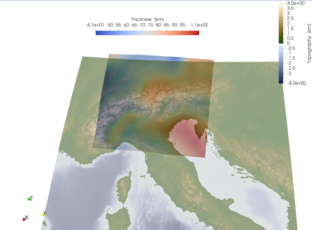
julia> write_paraview(Data_LM_lonlat, "Data_LM_lonlat")Opening and plotting the vertical field gives: