Visualisation

The standard visualisation way of GMG is to generate Paraview (VTK) files & look at them there. Yet, often we just want to have a quick look at the data without opening a new program. For that reason, we created the visualise widget, which uses GLMakie and allows you to explore the data.

It requires you to load both GLMakie and GeophysicalModelGenerator. A small example in which we load the tomography data of the alps is:

julia> using GeophysicalModelGenerator, GLMakie
julia> using GMT, JLD2

The last line loads packages we need to read in the pre-generated JLD2 file (see the tutorials) and download topography from the region. Lets load the data, by first moving to the correct directory (will likely be different on your machine).

julia> ;
shell> cd ~/Downloads/Zhao_etal_2016_data/      

Now you can use the backspace key to return to the REPL, where we will load the data

julia> Data = JLD2.load("Zhao_Pwave.jld2","Data_set_Zhao2016_Vp");    

At this stage you can look at it with

julia> visualise(Data);    

Note that this tends to take a while, the first time you do this (faster afterwards).

Let's add topography to the plot as well, which requires us to first load that:

julia> Topo = import_topo([0,18,38,52], file="@earth_relief_01m.grd");
julia> visualise(Data, Topography=Topo);    

Which will look like: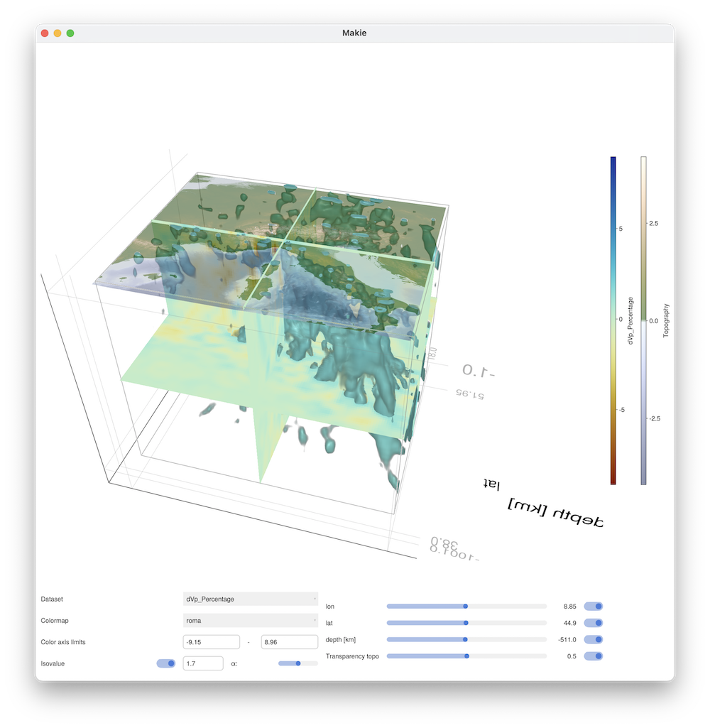

This is an example where we used GeoData to visualize results. Alternatively, we can also visualize results in km (often more useful for numerical modelling setups). For Visualize to work with this, we however need orthogonal cartesian data, which can be obtained by projecting both the data.

julia> p=ProjectionPoint(Lon=10, Lat=45)
ProjectionPoint(45.0, 10.0, 578815.302916711, 4.983436768349297e6, 32, true)
julia> Data_Cart  = CartData(xyz_grid(-600:10:600,-600:10:600,-1000:10:-1));
julia> Topo_Cart  = CartData(xyz_grid(-600:10:600,-600:10:600,0));
julia> Topo_Cart  = project_CartData(Topo_Cart, Topo, p)
CartData 
    size    : (121, 121, 1)
    x       ϵ [ -600.0 : 600.0]
    y       ϵ [ -600.0 : 600.0]
    z       ϵ [ -3.6270262031545473 : 3.654942280296281]
    fields  : (:Topography,)
  attributes: ["note"]
julia> Data_Cart  = project_CartData(Data_Cart, Data, p)
CartData 
    size    : (121, 121, 100)
    x       ϵ [ -600.0 : 600.0]
    y       ϵ [ -600.0 : 600.0]
    z       ϵ [ -1000.0 : -10.0]
    fields  : (:dVp_Percentage,)
  attributes: ["note"]

And once we have done that, you can visualize the data in the same way:

julia> visualise(Data_Cart, Topography=Topo_Cart)