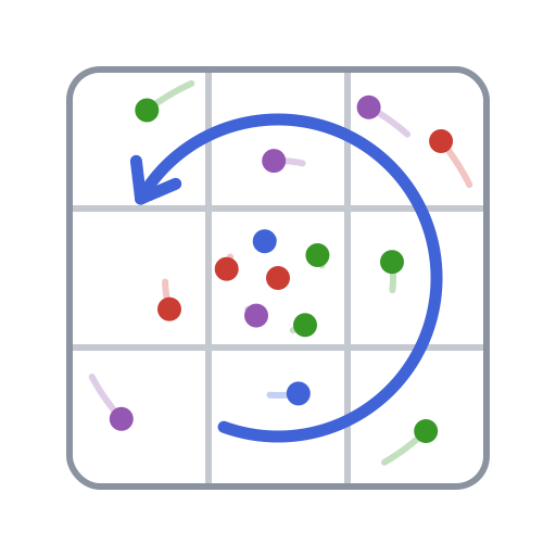
Particle lifecycle

Particles are stored by parent cell. A normal time step keeps that storage valid in four stages:

┌─────────────┐   ┌────────┐   ┌──────┐   ┌────────┐
│ interpolate │ → │ advect │ → │ move │ → │ inject │
└─────────────┘   └────────┘   └──────┘   └────────┘
       grid ↔ particle values        restore cell occupancy

grid2particle!(pT, T, particles)
advection!(particles, RungeKutta2(), V, dt)
move_particles!(particles, (pT,))
inject_particles!(particles, (pT,))
particle2grid!(T, pT, particles)

Initialize

Use a scalar nxcell for random, quadrant-balanced particles or a tuple for a regular layout:

particles = init_particles(backend, 24, 48, 12, grid_vx, grid_vy)
regular = init_particles(backend, (4, 4), 48, 12, grid_vx, grid_vy)
pT, = init_cell_arrays(particles, Val(1))

max_xcell reserves slots per cell; min_xcell controls reinjection. It is not a live-particle count. Use the occupancy mask when counting active slots.

Move and inject

advection! changes coordinates but does not reorganize cell storage. move_particles! relocates particles to their destination cells and moves companion fields with them. Particles that leave the domain or whose destination cell stays full can be removed; use verbose=true to report dropped particles.

inject_particles! restores occupancy using the particle fields supplied in its argument tuple:

move_particles!(particles, (pT,), verbose=true)
inject_particles!(particles, (pT,))

For phase-dependent injection, use inject_particles_phase!. Use clean_particles! when coordinates may no longer match their stored cells.

Phase injection accepts a tuple of grid fields with different layouts. Each field may be sampled at centers or vertices and may include one ghost sample per side on any axis. The layout is inferred separately from each field's size; all fields must use the particle grid's physical coordinates and precision. For example, inject_particles_phase!(particles, phases, (pT, pC), (T_center, C_vertex)) initializes both properties at each newly injected particle. Without ghost centers, boundary values use the nearest valid stencil and are clamped to its value range.

Both inject_particles!(particles, args, fields) and inject_particles_phase! take scheme = :grid (default) or scheme = :least_squares. The least-squares scheme fits a linear function to the particles that existed when the call started: in the new particle's cell, or in its 3^N neighborhood when the cell has too few. The result is clamped to the values carried by that neighborhood, and grid interpolation is used when no fit is possible. Particles injected by a call are never used as donors within that call, so the result does not depend on the order in which cells are processed.

inject_particles_phase!(particles, phases, (pT,), (T,); scheme = :least_squares)